A brief note on ellipse kinematics

Received: 28-Mar-2023, Manuscript No. PULJMAP-23-6280; Editor assigned: 30-Mar-2023, Pre QC No. PULJMAP-23-6280 (PQ); Reviewed: 13-Apr-2023 QC No. PULJMAP-23-6280; Revised: 29-May-2023, Manuscript No. PULJMAP-23-6280 (R); Published: 05-Jun-2023

Citation: Viktor S. A brief note on ellipse kinematics. J Mod Appl Phys 2023;6(3): 1-11.

This open-access article is distributed under the terms of the Creative Commons Attribution Non-Commercial License (CC BY-NC) (http://creativecommons.org/licenses/by-nc/4.0/), which permits reuse, distribution and reproduction of the article, provided that the original work is properly cited and the reuse is restricted to noncommercial purposes. For commercial reuse, contact reprints@pulsus.com

Abstract

The movement of a material point along curves of the second order is represented by the kinematic equation (1.10). The kinematics of second order curves is studied on an ellipse. Formulas for the dependence of acceleration and radius, speed and radius are derived. The direction of the velocity and acceleration vectors is determined. The conditions for the conservation of Kepler's laws when a material point moves along an ellipse are shown.

Keywords

Kepler's laws; Ellipse; Speed; Acceleration; Radius

Introduction

If simple equations of speed and acceleration are sufficient to describe rectilinear motion: V=S/t, a=S/t², then differential equations of motion are needed to solve problems on the curvilinear motion of material points and their systems. "The way we derive these equations doesn’t matter”: (1,§11,п. 3).

Formulas for the dependence of acceleration and radius, speed and radius

Point C moves in an ellipse relative to the focus (Figure 1).

Figure 1: For the dependence of acceleration and radius, speed and radius.

There is a system of equations for a parametric pendulum (1)

The parameter is time (t).

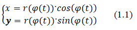
Let us substitute into system (1) the radius of the ellipse with respect to the focus:

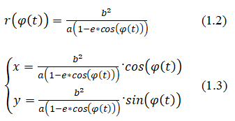
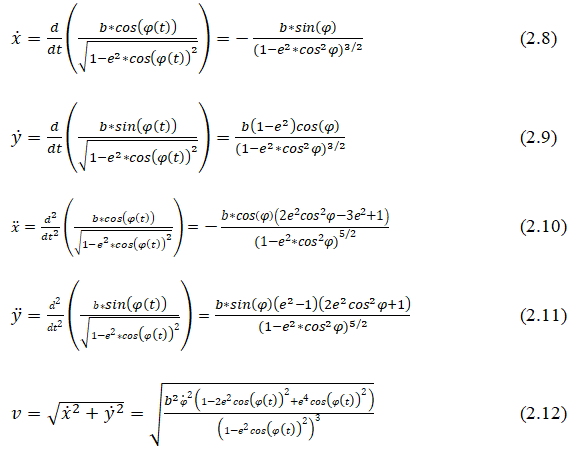
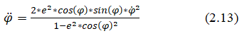
Let's differentiate twice. We get the coordinates of speed and acceleration:

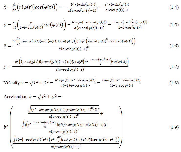
We form a system of equations from (1.6), (1.7) and solve for φ Ì?. We obtain the kinematic equation of motion of a point relative to the focus along second order curves:

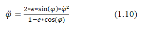
At different values of eccentricity, the shape of the curve will change [1].

We substitute (1.10) into (1.9), and simplify:

The sector speed is constant:

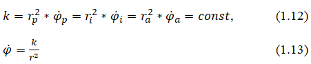
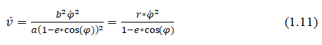
where r_p is the perifocal distance, r_a is the apofocal distance We substitute (1.13) into (1.11):

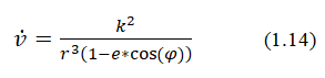
The acceleration v Ì? is recalculated using formula (14). Results (9) and (1 4) are compared (Figures 2 and 3).

Figure 2: Acceleration and radius.

We substitute (1.13) into (1.8):

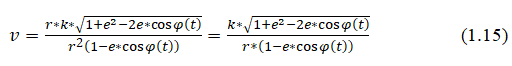
Figure 3: Velocity and radius.

Formulas (1.14, 1.15) do not give any advantage for calculating the modulus of speed and acceleration. First, to calculate the sector constant k, you need to calculate the angular velocity once. Secondly, in order for the motion of a point to comply with Kepler's laws, the angle must change according to elliptic equations. The value of these formulas is in the logical definition of the dependence of speed and acceleration on the radius [2].

Velocity and acceleration vectors

Let's consider two variants of point movement, Figure 4: a) Movement relative to the center; b) Movement relative to the focus.

Figure 4: Movement relative to the center and movement relative to the focus.

Note: v-speed, a-acceleration, dx, dy, ddx, ddy-first and second derivatives along the coordinate axes.

Note the property of collinear vectors on the plane rectangles built on vectors, Figure 5, should be similar:

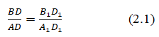
Figure 5: Rectangles built on vectors.

Movement relative to focus

Let's compare the ratio of the coordinates of the radius and acceleration:

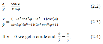
A special case of an ellipse.

In Figures 5–7 they are marked with red lines for speed, green for acceleration [3].

Coordinates of the beginning of the velocity and acceleration vectors, points of the initial ellipse (x,y). The coordinates of the end of the velocity vector (dx+x, dy+y). Acceleration vector end coordinates (ddx+x, ddy+y) [4].

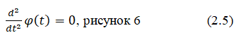
Figure 6: Coordinates of the beginning of the velocity and acceleration vectors.

Figure 7: The coordinates of the end of the velocity vector.

Movement relative to the center

To derive the kinematic equation of motion of a point relative to the center, we will replace the radius formula (2) with (13) in the system of equations (1.1) [5].

Let's differentiate twice. We get the coordinates of speed and acceleration:

We solve for φ Ì?. We obtain the kinematic equation of motion of a point relative to the center along second order curves:

Let's compare the ratio of the coordinates of the radius and acceleration:

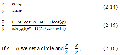
A special case of an ellipse, Figure 8.

Eccentricity e=0. Substitute in equation (2.15)

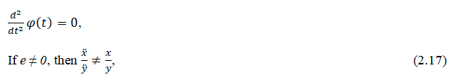
Figure 8: The ratio of the coordinates of the radius and acceleration.

Trammel of archimedes

Any point on the ellipsograph ruler moves along an elliptical path around the center.

In order not to refer the reader to the sources, we present the derivation of the formulas necessary for calculating velocities, accelerations, and rotation angles (Figure 9) [6].

Figure 9: The direction of the instantaneous rotation of the ruler AB around Р_АÐ? is clockwise in accordance with the direction of the known velocity vector of point A.

Ruler AB moves from horizontal to vertical position, Figure 9. Point C describes ¼ of the ellipse. The direction of the instantaneous rotation of the ruler AB around Р_АÐ? is clockwise in accordance with the direction of the known velocity vector of point A.

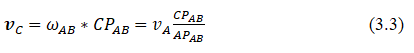
Speeds of points B and C:

Vector v_C is directed perpendicular to СР.

The directions of the velocities of the points and are determined by the instantaneous rotation of the ruler AB around the instantaneous center of velocities Р_АÐ?.

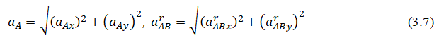
Determination of accelerations of points B and C

Let's use the theorem acceleration of points of a flat figure. Point A will be a pole, since the acceleration of point A is known.

The vector equation for the acceleration of point B has the form:

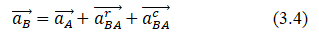
Where is the acceleration of the pole A (given);

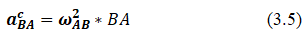
are the rotational and centripetal accelerations of the point B in the rotation of the ruler around the pole A. In this case:

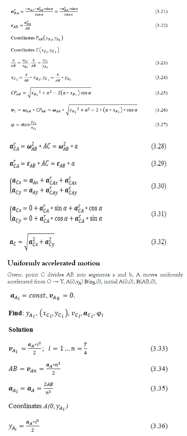
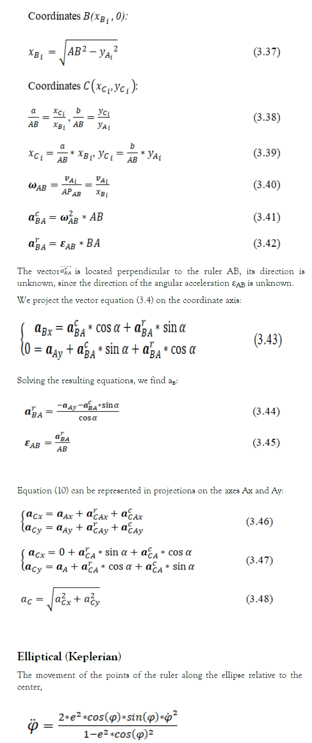
The vector is located perpendicular to the ruler AB, its direction is unknown, since the direction of the angular acceleration ε_AB is unknown.

In equation (3.4) there are two unknowns: Accelerations which can be determined from the equations of vector equality projections onto the directions of axes AX and AY:

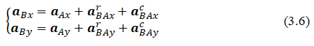
The direction of the vectors and is chosen arbitrarily. The solution of system (3.6) allows one to find the numerical value and with a plus or minus sign. A positive value indicates the correctness of the chosen direction of the vectors and a negative value indicates the need to change their direction (Figure 10).

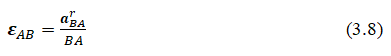
Ruler angular acceleration:

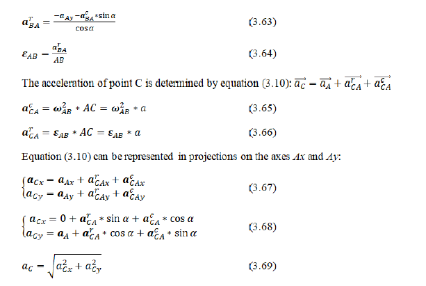
The acceleration of point C is determined by the equation:

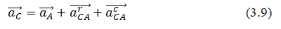
Figure 10: The rotational and centripetal accelerations of the point C relative to the pole A.

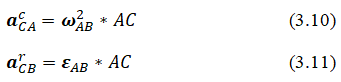
Where are, respectively, the rotational and centripetal accelerations of the point C relative to the pole A:

Equation (3.10) can be represented in projections on the axes Ax and Ay:

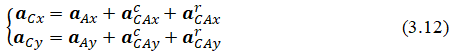
The acceleration projections of point C are determined from (3.10). The direction of the vector is determined by the signs of the projections ^aCx and ^aCy.

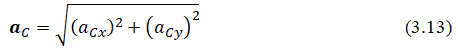
Vector modulus:

Let's take a look at the different travel options

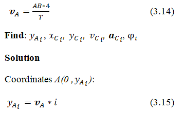
T is the period specified by arbitrary units of time. AB=a+b, A(0,y_A) Ð?(x_B, 0). Initial coordinates of points: A(0,0), Ð?(a+b,0), C(a,0). Initial speed v_A0=0.

Uniform movement

Given: point C divides AB into segments a and b, A(0,y_A), Ð?(x_B,0), initial A(0,0), B(AB,0). A moves uniformly from O → Y. Accelerations a_A=0, a_B=0, speed

Further, according to equations (3.4)–(3.14)

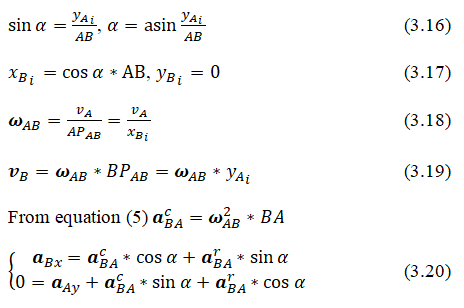
Solving the resulting equations, we find a_B,

Further, according to equations (3.4)–(3.14)

Given: point C divides AB into segments a and b, A moves elliptically according to the formula (2.13), from O → Y, A(0,yA), Ð?(xB,0), initial A(0,0), Ð?(AB,0),

The obtained motion parameters allow checking the fulfillment of Kepler's laws.

Kepler's second law

Equality of the areas of sectors is carried out only with elliptical motion (Figure 11-13).

Figure 11: Uniform movement.

Figure 12: Uniformly accelerated motion.

Figure 13: Elliptical (Keplerian) movement.

Graphical results of moving a point along an ellipse at different speeds (Figures 14-16).

Figure 14: Uniform movement.

Figure 15: Uniformly accelerated motion.

Figure 16: Elliptical (Keplerian) movement.

Kepler's laws as properties of kinematic equations of motion of a point along curves of the second order

The equations are solved by computer programs. The calculation results are compared with Kepler's laws. The uniqueness of the orbital velocity for the given parameters of the curve is noted. The orbital velocity is calculated from the kinematic equation and compared with the values of astronomical tables.

The sector velocity modulus is a constant for a given ellipse.

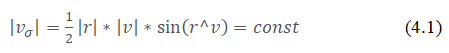
If a point moves along a flat curve and its position is determined by the polar coordinates r and φ, then

To illustrate the constancy of the sectoral velocity, a program was written to calculate the sector area in a given time interval. The program, TygeBraheKepler2_focal (A.1), calculates the parameters of the point movement according to equation (8) and shows the equality of the areas of the sectors at equal time intervals (Figures 17–19).

Figure 17: Shows the program test. The area of the ellipse is πab. 3.14159^*9^*7=197.92017.

Figure 18: Shows equal time intervals at different points in the period.

On Figure 19 added precession (dpi=0.1) to the parameters of Figure 18.

Figure 19: Shows the equality of the areas of the sectors at equal time intervals.

Kepler's third law

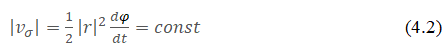
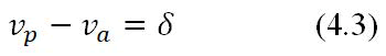
At perihelion and aphelion, sin(φ)=0, so the acceleration at these points is zero, and the modulo velocity difference is a constant:

Sector velocity according to the law of conservation of momentum is a constant value:

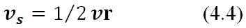
Let us express the sector velocity modulo the linear velocity.

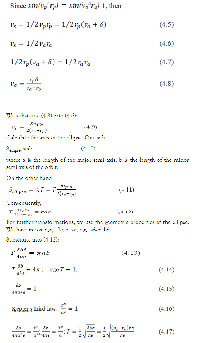
The program Movement of a mat point along an ellipse (A.2), using formulas (4.16) and (4.17), calculates the periods (Figures 20 and 21). δ=v_p-v_a(au/planet year).

Figure 20: The differential equation of the second order curves.

Figure 21: The differential equation of the second order curves with respect to the focus is calculated.

Differential equation of motion of a point along an ellipse with respect to the center

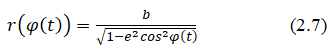
Let's move the origin of coordinates to the center of the ellipse, Figure 22. The radius function (2.7) will change.

Figure 22: The origin of coordinates to the center of the ellipse.

M-Material point. Q is a generalized force acting on a point. O-center, vlinear speed of the point. φ(t) is the angle between the X-axis and the point, counterclockwise.

Kepler's second law

The TygeBraheKepler2_center (A.1) program calculates the parameters of the point movement according to equations (2.7–2.13), and shows the equality of the areas of the sectors at equal time intervals (Figures 23–25).

Figure 23: Shows the program test. The area of the ellipse is πab. 2^*3.14159^*9^*7=197.92017

Figure 24: Equal time intervals are given at different moments of the period.

Figure 25: Added precession to the parameters.

On figure 25 added precession (dpi=0.1) to the parameters of figure 23.

Kepler's third law

The program movement of a mat point along an ellipse center (A.2), using formulas (4.16–4.17), calculates the periods. δ=v1–v2 (au/planet year).

In Figures 25-30 we see that with an increase in the eccentricity, the difference between the periods increases.

Figure 26: The program movement of a mat point along an ellipse center.

Figure 27: Increase in the eccentricity, the difference between the periods increases.

Figure 28: Shows the equality of the areas of the sectors at equal time intervals.

Figure 29: The motion of three or more bodies along second order curves.

Figure 30: For modeling streamlines of liquid and gas particles.

Conclusion

The kinematic equation (1.10) accurately describes the motion along ideal second order curves. The real orbits of cosmic bodies have deviations from the ideal curve: Precession, periodic asymmetry of the lengths of the radii, and other types of deviation.

Equation (1.10) and the center of mass theorem make it possible to simulate the motion of three or more bodies along second order curves.

The kinematic equation (2.13) is applicable for modeling streamlines of liquid and gas particles.

The article used materials from textbooks on mechanics.

References

1. Lilly JM. Kinematics of a fluid ellipse in a linear flow. Fluids. 2018;3(1):16.

   [Crossref] [Google Scholar]

2. Chiang CH. Spherical kinematics in contrast to planar kinematics. Mech Mach Theory. 1992;27(3):243-50.

   [Crossref] [Google Scholar]

3. Rubin-Delanchy P, Walden AT. Kinematics of complex valued time series. IEEE Trans Signal Process. 2008;56(9):4189-98.

   [Crossref] [Google Scholar]

4. Viviani P, Baud-Bovy G, Redolfi M. Perceiving and tracking kinesthetic stimuli: Further evidence of motor perceptual interactions. J Exp Psychol Hum Percept Perform. 1997;23(4):1232.

   [Crossref] [Google Scholar] [PubMed]

5. Shiller DM, Laboissiere R, Ostry DJ. Relationship between jaw stiffness and kinematic variability in speech. J Neurophysiol. 2002;88(5):2329-40.

   [Crossref] [Google Scholar] [PubMed]

6. Byrne JP, Gallagher PT, McAteer RT, et al. The kinematics of coronal mass ejections using multiscale methods. Astron Astrophys. 2009;495(1):325-34.

   [Crossref] [Google Scholar]