A high accurate method for solving an inverse problem of the Laplace equation in detection of a Robin coefficient

Abdelhak Hadj

doi:10.37532/2752-8081.22.6(4).9-13

Abdelhak Hadj^*

Higher National School of Renewable Energies, Environment and Sustainable Development, Algeria, Email: abdelhak.hadj@yahoo.com

^*Correspondence: Abdelhak Hadj, Higher National School of Renewable Energies, Environment and Sustainable Development, Algeria, Email: abdelhak.hadj@yahoo.com

Received: 16-Apr-2022, Manuscript No. puljpam-22-4949; Editor assigned: 23-May-2022, Pre QC No. puljpam-22-4949 (PQ); Accepted Date: Jul 12, 2022; Reviewed: 20-Jun-2022 QC No. puljpam-22-4949(Q); Revised: 29-Jun-2022, Manuscript No. puljpam-22-4949(R); Published: 15-Jul-2022, DOI: 10.37532/2752-8081.22.6(4).9-13

Citation: Hadj A. A high accurate method for solving an inverse problem of the Laplace equation in detection of a robin coefficient. J Pure Appl Math 2022;6(4):9-13

This open-access article is distributed under the terms of the Creative Commons Attribution Non-Commercial License (CC BY-NC) (http://creativecommons.org/licenses/by-nc/4.0/), which permits reuse, distribution and reproduction of the article, provided that the original work is properly cited and the reuse is restricted to noncommercial purposes. For commercial reuse, contact reprints@pulsus.com

Abstract

This study deals with an inverse problem for the harmonic equation to recover a Robin coefficient on a non-accessible part of a circle from Cauchy data measured on an accessible part of that circle. By assuming that the available data has a Fourier expansion, we adopt the Modified Collocation Trefftz Method (MCTM) to solve this problem. We use the truncation regularization method in combination with the collocation technique to approximate the solution, and the conjugate gradient method to obtain the coefficients, thus completing the missing Cauchy data. We recommend the least squares method to achieve a better stability

Keywords

Inverse problem; Ill-posedness; Robin Boundary Condition; Modified collocation; Trefftz method; Laplace equation

Introduction

The Laplace equation, usually named harmonic function, can be considered as a mathematical description for the study of several models describing various phenomena in the applied sciences, such as: temperature distributions, potentials of electrostatic, magneto-static fields, velocity potentials of incompressible irrotational fluid flows, the electrostatic problems, and in-compressible fluid [1-6]. Because of the powerful development of computers, considerable efforts have been made to solve Laplace’s equation in different shapes and boundary conditions [7].

The study of inverse problems became popular in modern science, and many problems governed by the harmonic equation can be considered as inverse problems. Nevertheless, these problems are generally illposed in Hadamard’s sense, because the existence, uniqueness and stability of the solution are not always guaranteed [8].

Problems governed by the Laplace equation are defined by their boundary conditions, for example the Dirichlet problem, the Neumann problem, the mixed or Direchlet-Neumann problem, and the Robin boundary value problem. For those problems where the appropriate boundary conditions are known on the entire boundary of the solution domain under consideration, these are direct problems. However, many experimental situations do not fall into this category due to physical difficulties or geometric inaccessibility. This is an important class of inverse problems known to be generally ill-posed.

Several methods are known for solving problems in applied sciences, such as: boundary integral equation methods (BIEMs), finite difference method (FDM), finite element method (FEM). The advantages and disadvantages of these methods are presented in [9]. Recently, Young, Chen and Kao (2007) proposed the Modified Collocation Trefftz Method (MCTM), which provides a very interesting method compared to the Collocation Trefftz Method (CTM) that renders convergent the series expansion of the solution and decreases the condition number of the discretization matrix [5, 10]. This approach has several applications for a large class of direct boundary value problems and also for inverse problems [11-14].

The Robin inverse problems are widely explored for the harmonic and also for the biharmonic equation. Their importance can be seen in many engineering applications such as, detection of the impedance and corrosion in electrostatic or thermal imaging, determine the Robin Coefficient/ Cracks’ Position in the steady-state heat conduction, the detection of specified functions in the elastic bending beam [3,11,15,16].

Numerous methods have been devoted to solve the Robin’s inverse problems, for example, the method of direct and indirect boundary integral equations, or by transform the problem in to an optimization problem based on the Fundamental Solution Method (MFS) [17-19]. It is important to point out that the reconstructions were taken at a small distance because the Robin’s problem for harmonic and Biharmonic equation are unconditionally solvable in the unit ball, and its solution is unique [15, 20].

In this paper, we will examine an inverse problem arising from electrical impedance tomography (EIT). Our goal is to describe a highly accurate method for determining the impedance information that may lie within a non-accessible part of the pipe, based on the measurement of electrostatic data on the accessible part of that pipe. We use the modified collocation Trefftz method proposed in to complete the missing Cauchy data, and the least squares method to achieve more stable results so as to recover the Robin coefficient [3].

Formulation of the problem

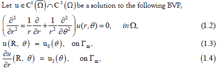
equation be an open disc of radius R, with circular boundary 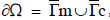where Γm and are two open disjoint portions of ∂Ω. By n we denote the outward unit normal to ∂Ω. Formulating the Laplace problem in the plane using plane polar coordinates has advantages, where Ω = {0 ≤ r < R, 0 ≤ θ < 2π},

equation

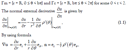
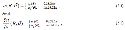
where e_r and e_θ are the polar coordinates of unit vectors [21]. It should be noted that, in order to make the Neumann data straightforward to calculate without losing generality, we restrict ourselves to a circle.

equation subject to the impedance boundary condition

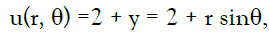
equation where p is an unknown function describing the contact impedance on the non-accessible part of the pipe, f is a given function can be taken as equal to zero, and u is the electrical potential [22-24]. The inverse problem we are consider with is to determine the impedance function p from the measurements of the voltage equation

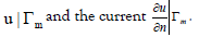
In [2,19] it presents that, if u0 and u1 are compatible on , then u is uniquely determined throughout Ω. Further, if p is non-negative then the direct problem is well posed and the uniqueness of solution is guaranteed. So we can use (1.5) to compute

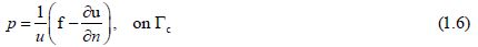Many articles are devoted to recover the Robin coefficients see [11, 14, 17, 18]. However, it should be pointed out that the solution u required a quantitative control of the possible vanishing. For example, if f = 0 and had a sign change, then u will vanish somewhere on ∂Ω, and this caused the equation (1.6) to become highly unstable. For the stability estimations we refer to the literature [1,2, 19].

To recover the Robin coefficient on a non-accessible part of the pipe. The remainder of this paper can be organized as follow: in section two, we require to perform a regularization of the accessible boundary data, to obtain a new collocation Trefftz method for the inverse Cauchy problem without needing for any iterations. We apply the modified collocation Trefftz method proposed in to obtain a non-ill-posed linear equations system can be solved with required accuracy by the conjugate gradient method to complete the messing Cauchy data [10]. The least square method is adopted in section three to recover the robin coefficient p on the non-accessible part of the pipe and we give examples to show the feasibility of this method, as a result, the conclusion is drawn.

The data completion problem

The collocation Trefftz method (CTM; i.e., the indirect TM), is popularly used in the engineering computations for the direct and inverse problems [10,25]. We are going to describe its modification and application for the two-dimensional Laplace equation and the inverse Cauchy problem to complete the messing Cauchy data, and to recover the Robin coefficient.

We replace the Equations. (1.3) and (1.4) by the following boundary conditions, respectively as:

equation

where ) are unknowns functions to be determined. We assume that 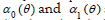are available to determine, then the Cauchy data are completed on the whole boundary, and the solution of Laplace equation can be obtained.

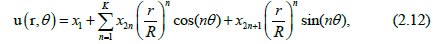
The numerical solution of the harmonic equation in a simply-connected domain is given by:

equation

where n c ,d ,n n ∈ Ν are unknown coefficients which will be retrieved uniquely by matching the boundary conditions (1.3-1.4). Indeed, by assuming that both functions equation and are L 2 integrable on the interval [0, bπ], then the uniqueness of u is guaranteed [10].

The F-Trefftz method, also called, the method of fundamental solutions (MFS), use the fundamental solutions as basis functions to develop the solution. In our article we used the MCTM to obtain a non-ill-posed linear equations system, this method is much simpler than that of the MFS, uses a very simple regularization of the input data by truncating higher modes see [5,10,25].

The T-complete bases functions for the two-dimensional Laplace equation in a simply connected domain can be shown as [10,12].

equation

In recent years, Liu has modified the T-complete functions by considering the characteristic length of the computational domain R to stabilize the numerical scheme by modifying the Trefftz method as follows [3,10]:

equation

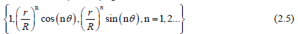
The characteristic length of the computational domain coincides with the radius of the pipe. We can recover the Trefftz method by taking R = 1 in (2.5). In the case of R > 1, the Trefftz method produces an unstable solution, whereas the modified Trefftz method is stable without any condition imposed on R. We view (2.5) as a modified collocation Trefftz method for expanding u in terms of T-complete functions of finite terms and replacing the infinite series in the original expressions by [10,15]

equation

The collocation method has a great advantage to apply on different geometric shapes, and the simplicity for computer programming. In order to apply the collocation method we define θ_i on Γ_m as:

equation

Matching the boundary conditions (1.3-1.4) on the equation (2.6). Afterwards, we have to apply the collocation (2.7) to obtain the non-ill-posed linear equations systems:

equation

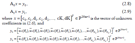
are the vectors obtains from values of the given functions 0 1 u ,u , respectively calculate at the collocations points (2.7). The matrix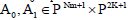 equation are given by

equation

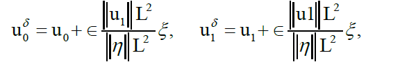
In general, both systems (2.8) and (2.9) are ill-posed [26] in the sense that a noisy data u^δ₀ ,u^δ₁are affected by a small arbitrary noise level δ as long as the following conditions are fulfilled:

equation

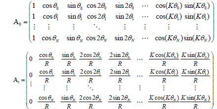
For the direct problem, we solve both systems (2.8) and (2.9) with required accuracy, to find the unknown coefficients in the equation (2.6). For this, it is sufficient to employ the conjugate gradient method. We get the following normal equation:

equation

In order to apply the MCTM on the inverse problem using Eq. (2.5) stability is the most important one of our interests. In the authors study the condition number for the matrix A0, A1 under different number of bases. They also present the advantages of the MCTM over the TCM. For accurate completion of the missing Cauchy data, we only consider the case where b ≥ 0.5 [10].

In what follows we use the conjugate gradient method to solve the normal equations (2.11) to complete the messing Cauchy data α₀, α₁ on [bπ, 2π]. Inserting the calculated x into Equation. (2.6) to obtain that

equation

and to complete the messing Cauchy data α₀, α₁on the following collocate points:

equation

Robin coefficients detection

To illustrate the high accuracy of the method presented in section (2), we show its feasibility to the inverse problem of recovering Robin coefficient. We see that, after having determined α₀, α₁ on the non-accessible part [bπ, 2π], then the Robin coefficient is obtained as a function in space from the following equation [17]:

equation

We compute the Robin function p at the collocation points (2.13) by solving

equation

In some instances, to achieve further stability in Eq. (1.6) under noisy data and to avoid dividing by small values of α₀ (θ_j) .We assumed that p can be represented by a linear combination of M appropriate basis functions as follows:

equation

where the basis equation can be chosen as the polynomials or the Gaussians as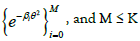 [27].

The design matrix B is a rectangular matrix of order equation with elements 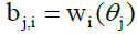In matrixvector notation, the residuals is given by:

equation

The least squares method consists in searching for the best approximation of p that makes the square sum of the residual in (3.4) as small as possible.

We solve the equation that is obtained by inserting (3.3) into (3.2) in the least squares sense for the coefficients αi a as follow:

In numerical examples we used cubic B-splines on an equidistant subdivision, here the collocation (2.13) is considered [28].

Numerical examples

In the stability of the data completion problem using MCTM is investigated when the boundary data is contaminated with noise (2.10) [10]. Several sets of noisy data have been generated in with noise added to the Dirichlet- Neumann data of the form [18].

equation

where ξ is a normally distributed random variable and is the relative noise level. Here, we present an examples show the reconstruction of Robin coefficient by the completion of messing Cauchy data using the MCTM [29].

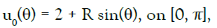
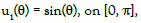
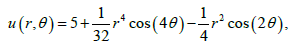
Example 1. In the first let Ω be the unique disc, and the exact solution is given by:

equation

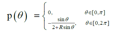
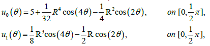
We can apply the MCTM on this example to obtain the data on the accessible boundary as

equation

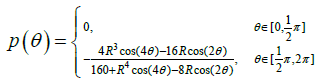
equation and the impedance profile

equation

We show the reconstructed profile for exact data and about 5% random noise added to the DirichletNeumann data (respect to the L2 norm) by using Nm = Nc = 150 collocate points with b = 1, and the regularized truncation number K = 6. In Figure 1 we compare the exact solution with it’s computed approximation for the exact data and for noise level ∈= 0.035. The errors were plotted in Figure 2 for the exact data and the noisy data. For the B-spline approximation of the impedance profile, the dimension M = 70 was used.

Figure 1: Reconstruction of the function profile p for a circle with radius R = 2.

Figure 2: Reconstruction of the function profile error under for a circle with radius R = 2.

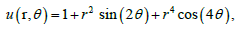
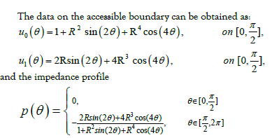
Example 2. In this example we consider a circle with radius R=3. The exact solution is taken as:

equation

The data on the accessible boundary can be obtained as:

equation

and the impedance profile

equation

This example, show the reconstructed profile for exact data and for 3% random noise added to the Dirichlet Neumann data (respect to the L2 norm) by using Nm = Nc = 130 collocate points with b = 0.5, and the regularized truncation number K = 4. In Figure 3 we compare the exact solution with the numerical solution for the exact data and for noise level ∈ = 0.07, the corresponding error was plotted in Figure 4 for exact data and for noisy data. We take M = 80 for the B-spline approximation of the Robin profile.

Figure 3: Reconstruction of the function profile p for a circle with radius R = 3.

Figure 4: Reconstruction of the function profile error under for a circle with radius R = 3.

Example 3. In this example we consider a circle with radius 1/2 = R , and the exact solution is given by:

equation

The following example, illustrate the reconstruction of the exact solution and for 4% random noise added to the Dirichlet-Neumann data (respect to the L2 norm) by using Nm=Nc= 130 collocate points with b = 0.5, and the truncation number K =4. In Figure 5 we compare the exact solution with the numerical solution for the exact data and for noise level ∈= 0.1. In Figure 6 we plot the errors, and we take M = 90 for the B-spline approximation of the Robin profile.

Figure 5: Reconstruction of the function profile p for a circle with radius R = 1.

Figure 6: Reconstruction of the function profile error under for an circle with radius R = 1.

Conclusion

We investigated the Robin inverse problem using the MCTM, the Cauchy data are given on the accessible part of the pipe and the Robin boundary condition is imposed on the non-accessible part of that pipe, in addition the Cauchy data are assumed to have Fourier expansions. We consider the finite truncation of the Fourier data to show the regularization of the inverse Cauchy problem, and the minimization to achieve stability.

As our interest is in inverse problems, we have seen that the MCTM provides a highly stable method that is straightforwardly compatible with the data completion problem. In particular, we have considered

The inverse Robin boundary value problem in a disk, where the solution of this inverse problem is highly accurate and robust against the noise.

References

- Alessandrini G, Del Piero L, Rondi L. Stable determination of corrosion by a single electrostatic boundary measurement. Inverse Probl. 2003;19(4):973-84.Google Scholar Crossref
- Chaabane S, Jaoua M. Identification of Robin coefficients by the means of boundary measurements. Inverse Probl. 1999;15(6):1425. Google Scholar Crossref
- Liu CS. Solving the Inverse Problems of Laplace Equation to Determine the Robin Coefficient/Cracks' Position Inside a Disk. CMES: Comput Model Eng Sci. 2009;40(1):1-28.Google Scholar Crossref
- Rundell W. Recovering an obstacle and its impedance from Cauchy data. Inverse Probl. 2008;24(4):045003.Google Scholar Crossref
- Li ZC, Lu TT, Hu HY, et al. Trefftz and collocation methods. WIT Press.2008.Google Scholar Crossref
- Jiang J, Zhou J. Analytical solutions of Laplace's equation for layered media in a cylindrical domain and its application in seepage analyses. Int J Mech Sci. 2020;184:105781.Google Scholar Crossref
- Morales M, Diaz RA, Herrera WJ. Solutions of Laplace's equation with simple boundary conditions, and their applications for capacitors with multiple symmetries. J Electrost. 2015;78:31-45.Google Scholar Crossref
- Tajani C, Abouchabaka J. On the data completion problem for Laplace's equation. Ann Univ Craiova-Math Comput Sci Ser. 2018;45(1):11-36.Google Scholar Crossref
- Brebia CA, Telles JCF, Wrobel LC. Boundary Element Techniques: Theory and Application in Engineering. Springer. 1984.Google Scholar Crossref
- Liu CS. A modified collocation Trefftz method for the inverse Cauchy problem of Laplace equation. Eng Anal Bound Elem. 2008;32(9):778-85.Google Scholar Crossref
- Hadj A, Saker H. Integral equations method for solving a Biharmonic inverse problem in detection of Robin coefficients. Appl Numer Math. 2021;160:436-50. Google Scholar Crossref
- Fan CM, Chan HF. Modified collocation Trefftz method for the geometry boundary identification problem of heat conduction. Numer Heat Transf B: Fundam. 2011;59(1):58-75.Google Scholar Crossref
- Ku CY, Xiao JE, Liu CY. On solving nonlinear moving boundary problems with heterogeneity using the collocation meshless method. Water. 2019;11(4):835.Google Scholar Crossref
- Cakoni F, Kress R, Schuft C. Integral equations for shape and impedance reconstruction in corrosion detection. Inverse Probl. 2010;26(9):095012.Google Scholar Crossref\
- Mera NS, Elliott L, Ingham DB, et al. An iterative boundary element method for the solution of a Cauchy steady state heat conduction problem. CMES: Comput Model Eng Sci. 2000;1(3):101-6.Google Scholar Crossref
- Slodička M, Van Keer R. A numerical approach for the determination of a missing boundary data in elliptic problems. Appl Math Comput. 2004;147(2):569-80.Google Scholar Crossref
- Cakoni F, Kress R. Integral equations for inverse problems in corrosion detection from partial Cauchy data. Inverse Probl Imaging. 2007;1(2):229-45.Google Scholar Crossref
- Cakoni F, Kress R, Schuft C. Simultaneous reconstruction of shape and impedance in corrosion detection. Methods Appl Anal. 2010;17(4):357-78.Google Scholar Crossref
- Wei T, Chen YG. Numerical identification for impedance coefficient by a MFS-based optimization method. Eng Anal Bound Elem. 2012;36(10):1445-52.Google Scholar Crossref
- Karachik VV. Solving a problem of Robin type for biharmonic equation. Russ Math. 2018;62(2):34-48.Google Scholar Crossref
- Ramm AG. A geometrical inverse problem. Inverse Probl.1986;2(2):19-21. Google Scholar Crossref
- Jiang Y, Soleimani M, Wang B. Contactless electrical impedance and ultrasonic tomography: Correlation, comparison and complementarity study. Meas Sci Technol. 2019;30(11):114001.Google Scholar Crossref
- Holder D. Electrical impedance tomography: methods, history and applications. Boca Rat FL: CRC Press. 2004. Crossref
- Kolehmainen V, Lassas M, Ola P. Electrical impedance tomography problem with inaccurately known boundary and contact impedances. IEEE Trans Med Imaging 2008;27(10):1404-14.Google Scholar Crossref
- Li ZC, Lu TT, Huang HT, et al. Trefftz, collocation, and other boundary methods—a comparison. Numer Methods Partial Diffe. Equ: Int J. 2007;23(1):93-144.Google Scholar Crossref
- Kita E, Kamiya N. Trefftz method: an overview. Adv Eng Softw. 1995;24(1-3):3-12.Google Scholar Crossref
- Li J. Application of radial basis meshless methods to direct and inverse biharmonic boundary value problems. Commun Numer Methods Eng.2005;21(4):169-82.Google Scholar Crossref
- Kress R. Numerical Analysis. Springer-Verlag New York. 1998.Crossref
- Watzenig D. Sequential Monte Carlo filter for two-dimensional reconstruction of material inhomogeneities in multiple phase flow fields; Sequenzielles Monte-Carlo-Filter zur zweidimensionalen Rekonstruktion von Materialinhomogenitaeten in Mehrphasenstroemungen. Tech Mess-TM. 2008;75(4):221–9.Google Scholar Crossref