A numerical approach for solving a class of fractional optimal control problems using Genocchi polynomials
2 Department of Applied Mathematics, University of Tabriz, Tabriz, Iraq
Received: 17-Apr-2024, Manuscript No. PULJPAM-24-7027; Editor assigned: 19-Apr-2024, Pre QC No. PULJPAM-24-7027 (PQ); Reviewed: 04-May-2024 QC No. PULJPAM-24-7027; Revised: 17-Mar-2025, Manuscript No. PULJPAM-24-7027 (R); Published: 25-Mar-2025
Citation: Moghaddam MA, Tabriz YE, Lakestani M. A numerical approach for solving a class of fractional optimal control problems using Genocchi polynomials. J Pure Appl Math. 2025;9(2):1-6.
This open-access article is distributed under the terms of the Creative Commons Attribution Non-Commercial License (CC BY-NC) (http://creativecommons.org/licenses/by-nc/4.0/), which permits reuse, distribution and reproduction of the article, provided that the original work is properly cited and the reuse is restricted to noncommercial purposes. For commercial reuse, contact reprints@pulsus.com
Abstract
In this paper, an efficient and accurate computational method based on the Genocchi polynomials is proposed for solving a class of fractional optimal control problems. In the proposed method, the Caputo fractional derivative operator for the Genocchi polynomials is given. The proposed technique is applied to transform the state and control variables into non-linear programing parameters at collocation points. The most important advantages of our method are easy implementation, simple operations. Some illustrative examples are presented to show the efficiency and accuracy of the method.
Keywords
Fractional optimal; Control problems; Caputo derivative; Genocchi polynomials; Operational matrix; Non-linear programming
Introduction
In the present paper, we consider a class of optimal control problems the objective function and the dynamic system with the Caputo fractional derivative as follows:
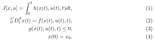
where h is a scalar function, x(t) is state vector and u(t) is control vector of dimension n × 1 and m × 1, respectively [1-3]. In the real word, many physical phenomena are controlled by the differential equations. Therefore, in recent years, Optimal Control Problems (OCPs) have been the interest of many scientists. A lot of research has been done in the context of OCPs, but the research on the Fractional Optimal Control Problems (FOCPs) is not so high. Ashpazzadeh, et al., in have used Hermite spline multiwavelest to solve the FOCPs. In, the ractional Remann-Liuovel is used to numerically solve the problem. Also, is a used numerical simulation for FOCPs with the Caputo fractional derivative in. In, Legandar functions are used as basis for solving FOCPs. Keshavarze used Bernoulli,s polynomials to solve FOCPs. Mashayekhi, et al., used hebrid functions basis to numerically solve FOCPs. The main aim of this paper is to solve fractional optimal control problems in the sense of Caputo derivative by using Genocchi polynomials. With the help of the Genocchi polynomials, the objective function, state and control vectors are expanded. To calculate coefficients, we used the collocation method with the nodes in the Chebyshev roots as collocation points. In finally, the FOCPs transformed into a problem with algebraic equations that can be solved by suitable algorithm. The paper is organized as follows: In the next section, we introduce the preliminary integration and fractional derivative. In section 3, we describe the basic formulating of the Genocchi polynomials required for our subsequent development. I section 4, we apply the Genocchi polynomials on [0, 1] to solve equations (1)-(4). In section 5, we will solve two numerical examples with the proposed method [4-6].
Materials and Methods
Some preliminaries in fractional calculus:
Here, we give two definitions related to Rieman-Liouvill fractional integral and Caputo fractional derivative.
Definition 1: The Riemann-Liouvill fractional integral of order β>0 of a function f is de- fined as follows:
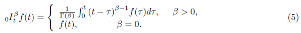
which Iβ is called the Riemann-Liouville fractional integration operator. Caputo,s derivative operator Dβ of a function f (t) is defined as follow:
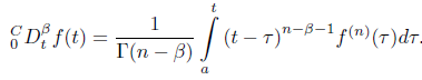
Definition 2: The Caputo fractional derivative of order β with the lower limit zero for a function
f ∈ Cn(0, ∞) is defined as follows. Some properties of Caputo, s fractional derivatives as:

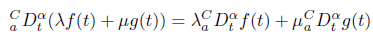
Where ⌈.⌉ is the ceiling function. Also the Caputo fractional-order derivative operator is a linear operator. That is, for all real scalers λ and μ and for all functions f (t) and g(t), we have:
Results and Discussion
Properties of Genocchi polynomials
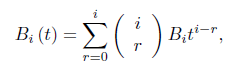
The genocchi polynomials: Suppose Gi(t) is the Genocchi polynomials that obtained from the formula below:
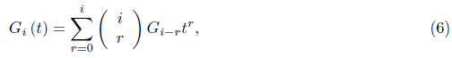
where Gi−r, r = 0, 1, . . . , i in Eq. (6) are the Genocchi numbers, that can be found as:
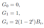
where Bi is the Euler, s numbers, which is defined as:

And
Thus, using Eq (6) and Genocchi numbers, we can write:
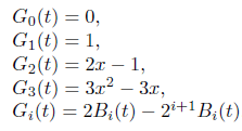
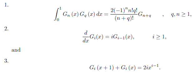
The set G(t) = G0(t), G1(t), . . . , Gn(t) is a complete orthogonal set in the Hilbert space L2[0, 1]. Thus, we can expand any functions in this space in terms of G(t) polynomials [7,8]. The Genocchi polynomials satisfies in the following relations:
The function approximation
Suppose G(t) is a N -vector as:

Function f (t) ∈ L2[0, 1] may be represented by the Genocchi polynomials as
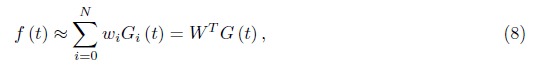
Where;
And, using Eq.(8) we obtain

Where;
Thus,

Operational matrices of fractional derivative
The kth derivative of G(x) is defined as:

Therefore, we can approximate derivative of arbitrary function f(t) using the Genocchi polynomials.
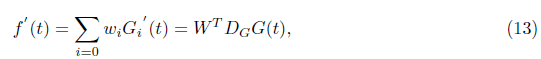
Where wi in Eq (13) is

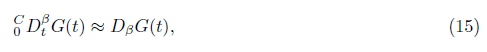
(i − 1) denotes the (i-1)th order derivative of f (t). In, for non-integer β > 0, the Caputo derivative of the vector G of order β can be defined as:
Where Dβ is a N × N matrix. It can be show:
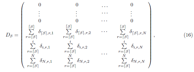
where ηi,k,j is given by:

Where Gi−r denotes the Genocchi numbers.
Sloving the fractional optimal control problems by the proposed method
In this section, we consider the FOCPs given in Eq (1)-(4). The factional state rate

state t vector x(t) and control vector u(t), can be approximated by Genocchi polynomials as:
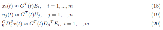
Where Dβ operational matrix given in Eq (16). We suppose:
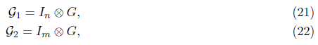
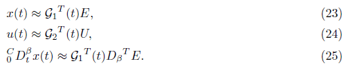
Im and In are m × m and n × n dimensional identity matrices, G(t) is N vector, ’⊗’ denotes Kronecker product and G1(t) and G2(t) are matrices of order mN × m and nN × n.
Then using Eqs (21, 22), we can write:
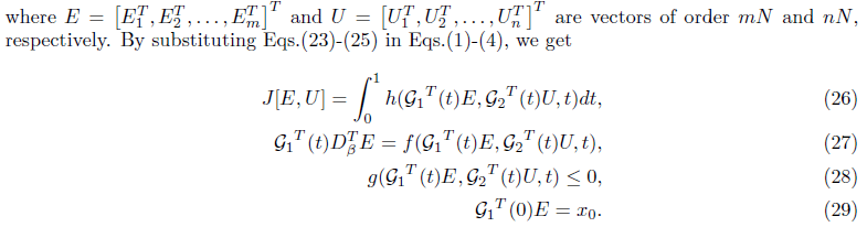
we assume two models for h in Eq (26):
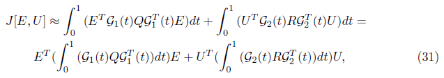
h(x(t); u(t); t) is quadratic function. Thus Eq (26) is to form:

Where T denotes transposition, Q is positive semi-definite matrix and R is the positive
definite matrix. Using Eqs (23, 24) we get:
Therefore;

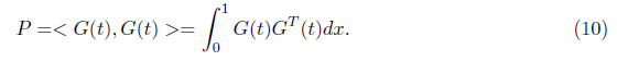
Using by Eq (10) we get:

h(x(t); u(t); t) is non-quadratic function. We evaluate objective function J by a suitable
Newton-Cots numerical integration as:
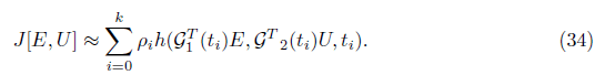
ρi, i = 0; 1; : : : ; k are the Newton-cots integration weight functions By collocating Eq (27) at the points:

We get

Now the problem changed to find the minimum solution of (33) or (34) with the conditions (29) and (36). Using lagrange multiplier method we have:
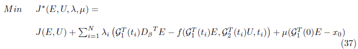
Where λ=(λ1, λ2, . . . , λN) and μ = (μ1, μ2, . . . , μN) are the lagrange multipliers. To find the optimal solution of Eq (37) we put

Eqs(38) given an algebraic system of equations which can be solved to find the values E, U, λ and μ [9-14].
Illustrative examples
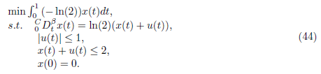
Example 1 consider the following free final state FOCPs:

With ptimal value J∗=0.171118. By applying present method, we obtain the numerical results (Table 1).
| Methods | J |
| Classical chebyshev | |
| m=8, k=26 | 0.17358 |
| m=16, k=28 | 0.17185 |
| Hybrid function | |
| w=15, m=3, n=4 | 0.170136 |
| w=15, m=4, n=4 | 0.170136 |
| Haar wavelet collocation | |
| K=8 | 0.172548 |
| k=16 | 0.171262 |
| k=32 | 0.170112 |
| Present method | |
| N=8 | 0.179078 |
| N=10 | 0.170291 |
| N=12 | 0.170049 |
TABLE 1 Comparison of the value of J for β=1, for example 1
values of N. Figure 1 shows the control function curves and plots of state vectors for β = 0.9, 0.99, 1 with N=10. Also, Table 1, shows the values of J for β=1 and gives a comparison between our results [15,16].
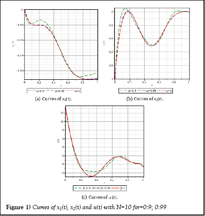
Figure 1) Curves of x1(t), x2(t) and u(t) with N=10 for=0:9; 0:99
Example: This example has been chosen from. The problem is:
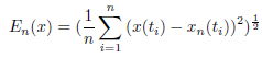
The state and control functions that minimize the preformance index J are given by x∗(t)=2t-1 and u∗(t)=1, respectively. This problem for β is adapted from e and has been studied by several authors. This problem has the minimum value objective function J∗=−0.30682 for β=1. Table 2, gives the results reported and the presented method. Also, Figure 2, (a) shows the plot of x(t) for exact value of state vector and approximate state vector where β approach to 1 and (b) shows plot of control vector for the different values of β, that approaches to 1 [17-20]. Also, for this problem, we define error of x(t), En(x), in the following from:
| Methods | J | En(x) |
| Method | ||
| n=2 | -0.3064 | 8.07e-4 |
| n=4 | -0.30682 | 4.99e-5 |
| n=8 | -0.30685 | 3.09e-6 |
| n=16 | -0.30669 | 1.92e-7 |
| n=32 | -0.30685 | 1.20e-8 |
| Method | ||
| M=3, N=1 | -0.30683 | - |
| Method | ||
| M=3, N=1 | -0.30684 | - |
| Method | ||
| M=3 | -0.30685 | - |
| Present method | ||
| N=5 | -0.30685 | 9.61e-6 |
| N=6 | -0.30685 | 2.98e â?? 6 |
| N=8 | -0.30685 | 3.21e â?? 9 |
TABLE 2 Comparison of the value of J for β=1, for example 2
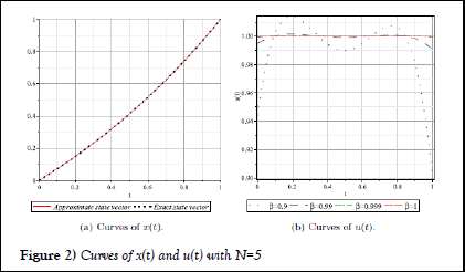
Figure 2) Curves of x(t) and u(t) with N=5
Conclusion
We demonstrated how to apply the Genocchi polynomials in the approximation of FOCPs. The developed technique proved to give accurate and consistent results for both the state and control variables. Computed errors between our approximate solutions and the analytical solutions of specific problems were negligible, proving the accuracy of our suggested scheme.
References
- Agrawal OP. A general formulation and solution scheme for fractional optimal control problems. Nonlinear Dyn. 2004;38:323-37.
- Agrawal OP. A formulation and numerical scheme for fractional optimal control problems. J Vib Control. 2008;14(9-10):1291-9.
- Agrawal OP. A quadratic numerical scheme for fractional optimal control problems. J Dyn Syst Meas Control. 2008;130(1).
- Agrawal OP, Baleanu D. A Hamiltonian formulation and a direct numerical scheme for fractional optimal control problems. J Vib Control. 2007;13(9-10):1269-81.
- Alipour M, Rostamy D, Baleanu D. Solving multi-dimensional fractional optimal control problems with inequality constraint by Bernstein polynomials operational matrices. J Vib Control. 2013;19(16):2523-40.
- Ashpazzadeh E, Lakestani M. Biorthogonal cubic Hermite spline multiwavelets on the interval for solving the fractional optimal control problems. Comput Methods Differ Equ. 2016;4(2):99-115.
- Baleanu D, Defterli O, Agrawal OP. A central difference numerical scheme for fractional optimal control problems. J Vib Control. 2009;15(4):583-97.
- Ghomanjani F. A numerical technique for solving fractional optimal control problems and fractional Riccati differential equations. J Egypt Math Soc. 2016;24(4):638-43.
- He Y. Some new results on products of the Apostol-Genocchi polynomials. J Comput Anal Appl. 2017;22(4):591-600.
- He Y, Araci S, Srivastava HM, et al. Some new identities for the Apostol–Bernoulli polynomials and the Apostol–Genocchi polynomials. Appl Math Comput. 2015;262:31-41.
- He Y, Kim T. General convolution identities for Apostol-Bernoulli, Euler and Genocchi polynomials. J Nonlinear Sci Appl. 2016;9(6):4780-97.
- Hosseinpour S, Nazemi A. Solving fractional optimal control problems with fixed or free final states by Haar wavelet collocation method. IMA J Math Control Inf. 2016;33(2):543-61.
- Isah A, Phang C. New operational matrix of derivative for solving non-linear fractional differential equations via Genocchi polynomials. J King Saud Univ Sci. 2019;31(1):1-7.
- Keshavarz E ordokhani Y, Razzaghi M. A numerical solution for fractional optimal control problems via Bernoulli polynomials. J Vib Control. 2016;22(18):3889-903.
- Lancaster P. Theory of Matrices, New York: Acad. 1969.
- Loh JR, Phang C, Isah A. New operational matrix via Genocchi polynomials for solving Fredholmâ?Volterra fractional integroâ?differential equations. Adv Math Phys. 2017;2017(1):3821870.
- Lotfi A, Dehghan M, Yousefi SA. A numerical technique for solving fractional optimal control problems. Comput Math Appl. 2011;62(3):1055-67.
- Lotfi A, Yousefi SA. Epsilon-Ritz method for solving a class of fractional constrained optimization problems. J Optim Theory Appl. 2014;163:884-99.
- Lotfi A, Yousefi SA, Dehghan M. Numerical solution of a class of fractional optimal control problems via the Legendre orthonormal basis combined with the operational matrix and the Gauss quadrature rule. J Comput Appl Math. 2013;250:143-60.
- Marzban HR, Razzaghi M. Hybrid functions approach for linearly constrained quadratic optimal control problems. Appl Math Model. 2003;27(6):471-85.