


 +447723598358

Advanced solutions to boundary value problems: A comparative study of Rayleigh-Ritz and the finite element method
Received: 11-Nov-2024, Manuscript No. PULJPAM-24-7317; Editor assigned: 13-Nov-2024, Pre QC No. PULJPAM-24-7317 (PQ); Reviewed: 27-Nov-2024 QC No. PULJPAM-24-7317; Revised: 17-Apr-2025, Manuscript No. PULJPAM-24-7317 (R); Published: 24-Apr-2025
This open-access article is distributed under the terms of the Creative Commons Attribution Non-Commercial License (CC BY-NC) (http://creativecommons.org/licenses/by-nc/4.0/), which permits reuse, distribution and reproduction of the article, provided that the original work is properly cited and the reuse is restricted to noncommercial purposes. For commercial reuse, contact reprints@pulsus.com
Abstract
This study investigates the solution of a boundary value problem using two numerical methods: The Rayleigh-Ritz method and the Finite Element Method (FEM). The aim is to compare the performance of these methods and assess the reliability of FEM as a generalization of the Rayleigh-Ritz approach for more complex problems. The Rayleigh-Ritz method and the linear element formulation of the finite element method were employed to solve the boundary value problem. A detailed comparison of the results obtained from both methods was performed. Graphical illustrations were used to present the solutions, and potential sources of error were analyzed, including element and domain approximation errors, round-off errors, and the impact of using linear rather than quadratic elements in FEM. The solutions generated by both methods were found to be in close agreement, demonstrating that FEM is a viable alternative to the Rayleigh-Ritz method for solving boundary value problems. The minor discrepancies observed can be attributed to approximation errors and the choice of linear elements in the finite element analysis. This work highlights the applicability and effectiveness of both the Rayleigh-Ritz method and FEM in solving boundary value problems. It underscores the finite element method’s flexibility, especially in handling more complex boundary conditions and geometries, and contributes to the understanding of the factors influencing the accuracy of numerical methods in structural analysis.
Keywords
Partial differential equations; Boundary value problem; Rayleigh Ritz method; Finite Element Method (FEM); Numerical analysis
Introduction
Mathematical models are essential in science and engineering for approximating and solving real-world problems. These models, which include linear, algebraic, and differential equations, help simulate and understand complex systems based on practical observations. In structural mechanics, they are crucial for predicting material stress, strain, and deformation in design and manufacturing. Numerical methods like the Finite Element Method (FEM) have become indispensable for solving such models, particularly for problems involving complex domains, varying material properties, or nonlinear behaviors that make analytical solutions challenging.
The FEM provides approximate solutions by discretizing a system into smaller, manageable parts called finite elements. This subdivision allows for accurate representation of complex geometries and is computationally efficient. However, while FEM is widely applied, its comparative performance as a generalization of other methods, such as the Rayleigh-Ritz method, particularly in terms of approximation accuracy and computational efficiency, is a topic of continued research.
Research objectives
This study aims to address the following questions:
• How do the Rayleigh-Ritz and finite element methods compare in solving boundary value problems?
• What are the sources of error in each method, and how do they affect the accuracy of the solutions?
• To what extent can the use of linear elements in FEM impact the overall performance in comparison to the Rayleigh-Ritz method?
Scope and methodology
The study will involve solving a boundary value problem using both the Rayleigh-Ritz method and the linear element approach of the finite element method. The accuracy of the approximations will be compared through graphical illustrations and numerical analysis. Sources of error, including element approximation and domain discretization, will be identified and evaluated. While FEM will be explored using linear elements, more advanced elements such as quadratic or cubic will not be considered in this analysis. Additionally, the study will focus solely on static, linear problems and will not account for dynamic or nonlinear behavior, which could be addressed in future research.
Materials and Methods
Weighted integrals
In almost all approximate methods used to determine the solution of differential and integral equations, we seek a solution in the form
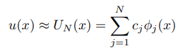
where u represents the solution of a differential equation and associated boundary conditions, and UN is its approximation that is represented as a linear combination of unknown parameters cj and known functions ϕj of position x in the domain Ω on which the problem is posed. We shall shortly discuss the conditions on ϕj. The approximate solution UN is completely known only when cj are known. Thus, we must find a means to determine cj such that UN satisfies the differential equation at every point x of the domain Ω and conditions on the boundary Γ of Ω, then UN (x) = u(x),
which is the exact solution of the problem. Of course, approximate methods are not about problems for which exact solutions can be determined by some methods of mathematical analysis: The role of approximate methods is to find an approximate solution of problems that prove difficult to obtain analytically.
When the exact solution cannot be determined, the alternative is to find a solution UN that satisfies the governing equations in an alternative way. In the process of satisfying the governing equations approximately, we obtain (not accidentally but by planning) N algebraic relations among the N parameters c1, c2, . . . , cN. For example, consider the problem of solving the differential equation

subjected to the boundary conditions
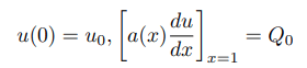
where a(x), c(x), and f(x) are known functions, u0 and Q0 are known parameters, and u(x) is the function to be determined. We now seek an approximate solution over the entire domain Ω=(0, L) by substituting UN into equation 1 such that

We shall consider how to solve such equations later. The equation requires the approximate solution UN to satisfy the differential equation in the weighted-integral sense,

Development of weak forms
There are three steps in the development of the weak form of any differential equation.
Step 1: This step is the same as in a weighted-residual method. Move all terms of the differential equation to one side (so that it reads . . . = 0), multiply the entire equation with a function w(x), and integrate over the domain Ω=(0, L) of the problem

Recall that the expression in the square brackets is not identically zero since u is replaced by its approximation, UN. Mathematically, in equation 2, the error in the differential equation (due to the approximation of the solution) is made zero in the weighted integral sense.
Step 2: While the weighted integral statement, equation 2, allows us to obtain the necessary number (N) of algebraic relations among cj for N different choices of the weight function w, it requires that the approximation functions ϕj be such that UN is differentiable as many times as needed in the original differential equation and satisfies the specified boundary conditions. So, it makes sense to shift half of the derivatives from u to w so that both are differentiated equally, and we have weaker continuity requirements on ϕj. The resulting integral form is known as the weak form [1,2].
Step 3: The third and last step of the weak formulation is to impose the actual boundary conditions of the problem under consideration. It is here that we require the weight function w to vanish at boundary points where the essential boundary conditions are specified, i.e., w is required to satisfy the homogeneous form of the specified essential boundary conditions of the problem [3,4].
Linear and bilinear functional
Linear and bilinear functionals are fundamental concepts in functional analysis and variational methods, including the Rayleigh-Ritz method, which is used to approximate solutions to Boundary Value Problems (BVPs). These functionals play a key role in formulating and solving the variational form of the governing differential equations. A linear functional L maps a function u from a vector space into real numbers R, such that:

for any scalars c1, c2 and functions u1, u2. In the Rayleigh-Ritz method, linear functionals are typically associated with external forces, boundary conditions, or source terms in the governing equations. A bilinear functional, B(u,v), maps two functions u and v from a vector space into real numbers R, and it is linear in each argument [5]:

for any scalars c1, c2 and functions u1, u2, andv. In boundary value problems, bilinear functionals often represent the energy terms in the system, such as the potential energy in elasticity or other physical quantities. The Rayleigh-Ritz method is based on variational principles, where the objective is to minimize a functional (often representing the total energy of the system) to find an approximate solution to a BVP. This is done by approximating the solution as a linear combination of trial functions and applying the variational principle. In the variational formulation of a boundary value problem, the solution satisfies a weak form of the governing differential equations. This weak form is expressed using bilinear and linear functionals as shown below
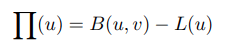
where (u) is the second-order differential equation for the system, B(u,v) is the bilinear functional representing the system’s internal energy, and L(u) is the linear functional representing external forces. In the Rayleigh-Ritz method, the trial solution u(x) is expressed as a linear combination of known basis functions ϕi(x):
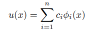
where ci are unknown coefficients to be determined. Substituting this into the variational form leads to a system of algebraic equations for ci, which are obtained by minimizing the functional [6]:
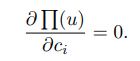
These functionals transform the original problem into an optimization problem, where the weak form is minimized to approximate the solution.
A brief look at the finite element method
The Finite Element Method (FEM) is a numerical technique for solving problems which are described by partial differential equations. The finite element method is a technique in which a given domain is represented as a collection of simple domains, called finite elements, so that it is possible to systematically construct the approximation functions needed in a variational or weighted-residual approximation of the solution of a problem over each element. Thus, the finite element method differs from the traditional Ritz, Galerkin, least-squares, collocation and other weighted residual methods in the manner in which the approximation functions are constructed. But this difference is responsible for the following three basic features of the finite element method [7]:
• Division of whole domain into sub-domains that enable a systematic derivation of the approximation functions as well as representation of complex domains.
• Derivation of approximation functions over each element.
• Assembly of elements is based on the continuity of the solution and balance of internal fluxes; the assemblage of elements results in a numerical analog of the mathematical model of the problem being analyzed.
Discretization of the domain: In the finite element method, the domain Ω of the problem is divided into a set of subintervals i.e., line elements, called finite elements. A typical element is denoted Ωe and it is located between points A and B with coordinates xa and xb (i.e., of length xb−xa). The reason for dividing a domain into a set of sub-domains is twofold. First, domains of most systems by design are a composite of geometrically materially different parts, and the solution on these sub-domains is represented by different functions that are continuous at the interfaces of these sub-domains. Therefore, it is appropriate to seek approximation of the solution over each sub-domain. Second, approximation of the solution over each element is simpler than its approximation over the entire domain. However, the number of elements into which the total domain is divided in a problem depends mainly on the geometry of the domain and on the desired accuracy of the solution [8].
Derivation of element equations: In the finite element method, we seek an approximate solution to equation 1 over each finite element. The polynomial approximation of the solution within a typical finite element Qe is assumed to be of the form

where uje are the values of the solution u(x) at the nodes of the finite element Qe, and are the approximation functions over the element. Next, we develop the algebraic equations among the unknown parameters, like the Ritz and Galerkin method. The main difference here is that we work with a finite element (i.e., sub-domain) as opposed to the total domain. This step results in a matrix equation of the form [Ke] {ce} = {Fe}, which is called the finite element model of the original equation. The derivation of finite element equations involves the following three steps:
• Construct the weighted-residual or weak form of the differential equation.
• Obtain an approximate solution over a typical finite element.
• Derive the finite element equations by substituting the approximate solution into the weighted- residual or weak form [9].
To obtain the weak form, we multiply the governing differential equation 1 with a weight function w and integrate over a typical element which results into

The last step is to identify the primary and secondary variables of the weak form. This requires us to classify the boundary conditions of each differential equation into essential (or geometric) and natural (or force) boundary conditions. The classification is made uniquely by examining the boundary term appearing in the weak form (equation 6),
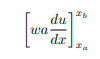
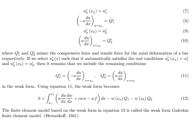
The coefficient of the weight function w in the boundary expression is called a secondary variable. The dependent unknown u in the same form as the weight function w appearing in the boundary expression is termed a primary variable. For the model at hand, the primary variable is u while the secondary variable is adu/adx. For a typical lone element, we have four boundary conditions
Assemblage of element: The final aspect of finite element analysis is to assemble all the finite elements. In deriving the element equations, we isolated a typical element (the eth element) from the mesh and formulated the variational problem (or weak form) and developed its finite element model. To obtain the finite element equations of the total problem, we must put the elements back into their original positions. In putting the elements with their nodal degrees of freedom back into their original positions, we must require that the solution u(x) is uniquely defined (i.e., u is continuous) and their source terms Qie are balanced at the points where elements are connected to each other. Please note, if the variable u is not continuous, we do not impose its continuity; but in the problem studied the primary variable is assumed to be continuous (r5). The assembly of elements is carried out by imposing the following two conditions:
If the node i of element Ωe is connected to the node j of element Ωf and node k of element Ωg, the continuity of the primary variable u requires

For the same three elements, the balance of secondary variables at connecting nodes requires

where I is the global node number assigned to the nodal point that is common to the three elements and QI is the value of externally applied source, if any (otherwise zero).
Main section
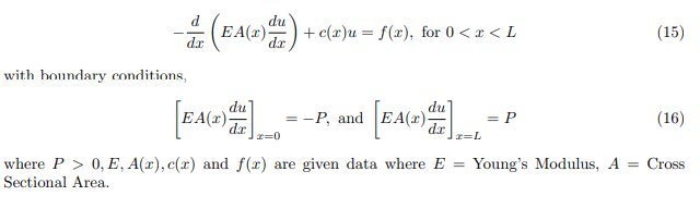
In this study, we shall consider a boundary value problem as given in the equation below:
Variational method for solving boundary value problems (Ritz method)
To approach this problem, we choose the approximate solution in the form
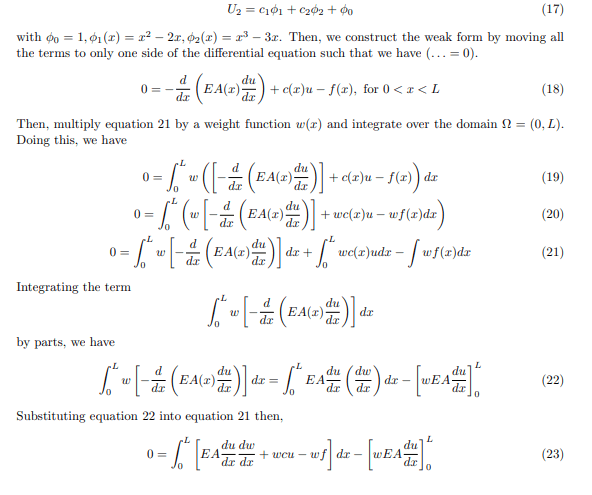
Applying our boundary conditions,

Equation 24 is called the weak form of the equation. The word weak refers to the weakened continuity of u, which is required to be twice differentiable in the weighted integral statement equation 21 but only once differentiable in equation 24.
The variational problem and quadratic functional can be expressed in the form:
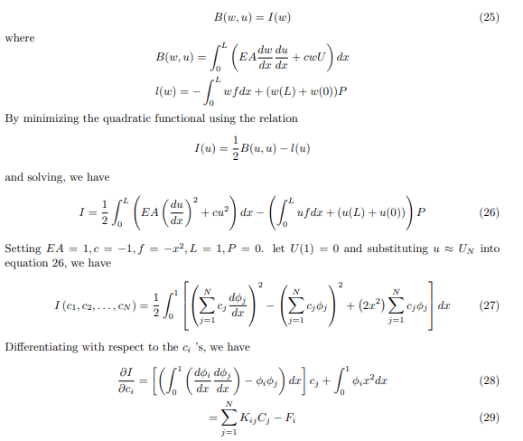
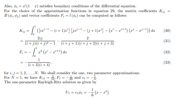

Solving the linear equation using Crammer’s rule, we obtain c1=−0.08197, c2=−0.16939 The two parameter Ritz solution is given by:

Using the finite element analysis
We recall the problem
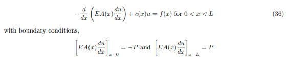
where P>0, E, A(x), c(x) and f (x) are given data.
We divide the domain over two subdivisions i.e., we have two finite elements. Using the Ritz method, we obtain the weak form over each subdivision which is given as
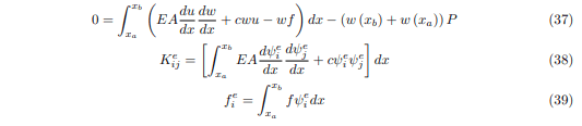
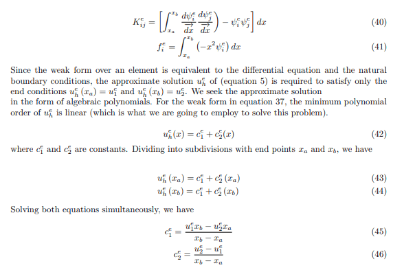
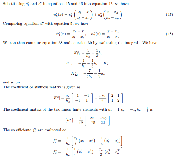
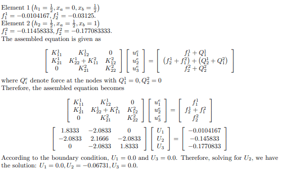
Following our previous assumption, we set EA=1, c=−1, f=−x2, L=1, P=0. The coefficient matrix over a finite element is given as
Results
The results indicate that the three approaches Ritz solutions using one and two parameters, as well as the finite element method with two subdivisions exhibited similar convergence behavior. The solutions are relatively close to one another, and the observed variations can be attributed to the simplifications and assumptions made during the modeling process. In the case of the Ritz method, increasing the number of parameters used in the calculations leads to enhanced accuracy of the results. This is because a higher number of parameters captures the underlying complexities of the boundary value problem more effectively. Similarly, for the Finite Element Method (FEM), employing higher-order polynomials within the elements can significantly improve the accuracy of the solutions. Higher-order polynomials provide a more flexible framework for representing the solution over each element which enables better approximation of complex behaviors. Overall, while both methods demonstrate effective convergence, the choice of parameters and polynomial order plays a crucial role in determining the precision of the final solutions. Future analyses could explore the impact of varying these parameters further, potentially leading to even more accurate and reliable results in solving boundary value problems (Figures 1 and 2).
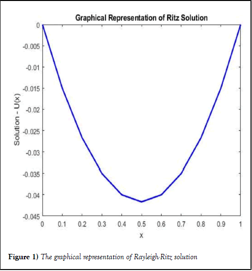
Figure 1) The graphical representation of Rayleigh-Ritz solution
| x | Ritz Solution | FEM | |
| N=1 | N=2 | Linear element | |
| 0 | 0 | 0 | 0 |
| 0.1 | -0.0015 | -0.0089 | -0.0135 |
| 0.2 | -0.0267 | -0.0185 | -0.0269 |
| 0.3 | -0.035 | -0.0279 | -0.0404 |
| 0.4 | -0.04 | -0.0359 | -0.0538 |
| 0.5 | -0.0417 | -0.0417 | -0.0673 |
| 0.6 | -0.04 | -0.0441 | -0.0538 |
| 0.7 | -0.035 | -0.0421 | -0.0404 |
| 0.8 | -0.0267 | -0.0348 | -0.0269 |
| 0.9 | -0.015 | -0.0211 | -0.0135 |
| 1 | 0 | 0 | 0 |
Table 1) Comparison between the solutions of Rayleigh-Ritz and finite element methods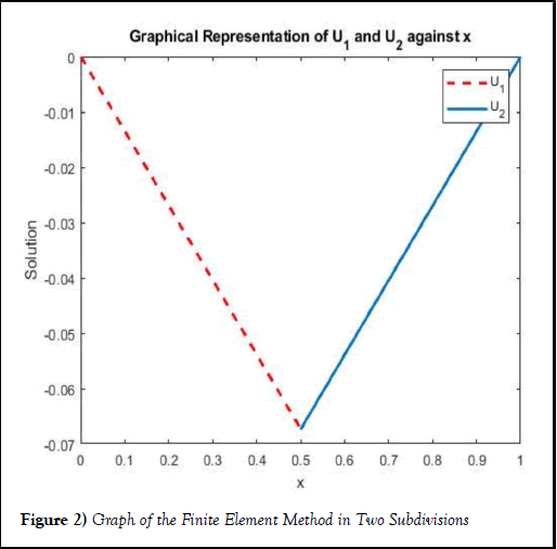
Figure 2) Graph of the Finite Element Method in Two Subdivisions
Discussion
A systematic study of the steps involved in the finite element formulation of a model second-order differential equation in a single variable was presented. The study introduces the basic principles of the finite element method and applied them to uni-dimensional problems. Taking a close look at Table1, we discover that the values obtained using the finite element method are reasonably close to those obtained using the Ritz method. This shows that the finite element method is equivalent to the use of the Rayleigh-Ritz method with a piecewise polynomial approximation to the displacement. The approximation is defined through a finite set of nodal values that constitute the degrees of freedom of the problem.
Conclusion
In using the finite element method, the use of quadratic element is highly recommended for higher studies compared to the use of linear element for a better and more accurate solution. Also, in this research work, the domain was divided into two subdivisions to avoid too much computation. It is recommended that the domain be split into as many subdivisions as possible.
Acknowledgment
I appreciate Dr. Samuel A. Borokinni for his supervision of this paper and his invaluable support and guidance throughout the research process. Dr. Borokinni went above and beyond, dedicating countless extra hours to ensure that this document met the highest standards. I am truly grateful for his unwavering commitment and mentorship.
References
- Babuska I. Survey lectures on the mathematical foundations of the finite element method. 1972:3–359.
- Courant R. Variational methods for the solution of problems of equilibrium and vibrations. 1994:1–11.
- Hrennikoff A, Kiritsis D. Engineering Asset Management: Proceedings of the Fourth World Congress on Engineering Asset Management (WCEAM) 2009. Springer Science & Business Media; 2011.
- Logan DL. A first course in the finite element method. 2011.
- Reddy JN. An introduction to the finite element method. 1993.
- Belayev WB, Tsipenyuk Dâ?¯Yu. Gravi electromagnetism in five dimensions and moving bodies in Galaxy area. Spacetime Subst. 2004;22:49.
- Yun YH, Jang K, Sung YK. Unification of gravitational and electromagnetic fields using gauge symmetry. J High Energy Phys Grav Cosm. 2021;7(1):106924.
- Breban R. Electromagnetism from 5D gravity: beyond the Maxwell equations. Eur Phys J Plus. 2021;136:440.
- Kawai T. A five dimensional unification of the vierbein and electromagnetic fields. II: geometric structure with regard to affine connection of the bundle space. Prog Theor Phys. 1982;68(4):1365-76.