An Event Graph in Special Relativity

Received: 14-Jun-2023, Manuscript No. puljmap-23-6556; Editor assigned: 26-Jun-2023, Pre QC No. puljmap-23-6556(PQ); Accepted Date: Jul 08, 2023; Reviewed: 29-Jun-2023 QC No. puljmap-23-6556(Q); Revised: 04-Jul-2023, Manuscript No. puljmap-23-6556(R); Published: 10-Jul-2023, DOI: 10.37532.2023.6.3.1-5

Citation: Hokstad P. An Event Graph in Special Relativity. J Mod Appl Phys. 2023; 6(3):1-5.

This open-access article is distributed under the terms of the Creative Commons Attribution Non-Commercial License (CC BY-NC) (http://creativecommons.org/licenses/by-nc/4.0/), which permits reuse, distribution and reproduction of the article, provided that the original work is properly cited and the reuse is restricted to noncommercial purposes. For commercial reuse, contact reprints@pulsus.com

Abstract

We present a graph to illustrate a series of events within the theory of special relativity. This spacetime diagram provides both the so-called proper time and calendar time, in addition to one space parameter. All parameters of the graph are given in time units, and we also relate the graph to a time vector in two dimensions. The approach considers chains of events having a piecewise constant velocity and is exemplified, e.g. by versions of the twin paradox

Key Words

Spacetime diagram, event graph, time vector, internal clock, twin paradox, µ-mesons

Introduction

First, we suggest a graph, describing an object with constant velocity, (in its simplest form suggested in Ref 1 then generalizing it; allowing the velocity to be piecewise constant [1]. This event graph is a spacetime diagram; somewhat analogous to the ‘world line’ of Minkowski Ref,2, Here we use the so-called proper time and the position (in time units) as the two main parameters of the diagram[2].

However, the calendar time is also provided. We apply the graph to variations of the travelling twin example. Also, the case of the µmesons is used as an illustration

1. Basic Notation and the Time Vector

We start out with a Reference Frame (RF), denoted K, and now restrict to one space coordinate, x. This RF has synchronized, stationary clocks located at virtually any position. Further, there is an object moving at a constant velocity, w, relative to K, along the x-axis. This moving object (is imagined to) bring with it a clock, which is synchronized with the clocks on K at an initial position.

The three fundamental parameters related to the movement of this object are: τ = Clock reading of the clock following the moving object. This is usually referred to as the proper time, and can also be seen as the ‘internal time’ of the object/event; x = Position of the moving object relative to K, (when the passing clock reads τ); t = Clock reading of the clock permanently located at position x on K, when the moving clock reads τ; this t is usually referred to as calendar time.

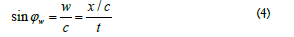
Letting the object start out from the position x = 0 at time t = 0, the velocity of the object relative to the RF, K equals W = x/ t, and as usual c = speed of light. Then - according to the so-called time dilation in special relativity - we have

The parameters (t, x) specify an event relative to the chosen RF, and we introduce a time vector related to the event (t, x):

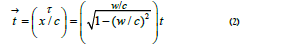
This vector has absolute value

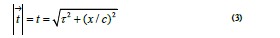
Thus, all three parameters τ,t and x/c represent time. In particular, x/c equals the time required for light to traverse the distance x. We can interpret t as the total ‘distance’ (in time) from the initiating event, (t = 0, x = 0), and so Eq. (3) provides a decomposition of this t into its two components, t and x/c. We see that the time vector in Eq. (2) comprises the information of all the above fundamental parameters of an event; including the velocity, w, as specified by the angle 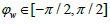through

2. A Simple Event Graph

We now consider a simple graph to describe the series of events, as specified by the moving object.

2.1 Specification: Figure 1 provides a graphical illustration of all four parameters: t, x/c, t and w of a specific event; also demonstrating how they are related. In particular, the two components of the time vector are given as, see Eqs. (1) - (4):

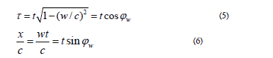
Figure 1:An ‘event graph’: A chain of events, on a specific RF; describing an object of constant velocity, w relative to this RF

But, in addition to provide the time vector of a specific instant, this line also illustrates the whole chain of events, representing the object’s movement from time 0, and we then denote this an event graph.

2.2 Examples: We illustrate the above graph with a couple of standard examples.

Example 1. The twin paradox The travelling twin example is discussed by a number of authors, Refs. [3, 4]. We apply a rather standard numerical example, letting the travelling twin leave the earth in a rocket of velocity, w = 0.6c, giving He travels to a ‘star’ located 3 light years from the earth. This means that x/c = 3 years, and by this arrival to the star, the (imagined) clock permanently located at the star reads t = x/w = 3c/0.6c = 5 years.

According to special relativity, the travelling twin’s clock will at this instant read, see Eq. (1),

In summary, by the arrival of the rocket to the star, we have t = 4 years, x/c = 3 years, t = 5 years. Or, expressed by the time vector of this even, (see the line OB of Figure. 2.a)):

Figure 2: Examples of event graphs, (both in the perspective of the earth)..

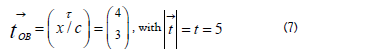
Here O represents the travelling twin’s start of the travel from the earth, and B is the event of his arrival to the star. In this figure we have also inserted two other event graphs. First, the red line OA, illustrates the clock of the brother who remains on the earth, (having x/c ≡ 0); and finally, the line CD, illustrates the (imagined) clock permanently situated on the star.

These three event graphs are related to the RF of the earth; all starting simultaneously with t=τ=0, (at events O and C, respectively). So, in the perspective of this RF, the figure gives the three time vectors, which also represent three simultaneous chains of events. We note that the event B, representing the end point of OB, and event D, representing the end point of CD, might be seen as two equivalent eventss, as they have the same t = 5, and the same x/c = 3 relative to the chosen RF. However, they are not fully equivalent; as they are not represented by the same time vector, (having different w's). This stems from the fact that they represent events chains, starting out from different positions, (and having different w’s). This will also cause us to provide different predictions for the two event chains, occurring after this single common event,(t=5,x/c=3)

Example 2. The Mu-mesons.

This is another standard example, typically described [5]. The µmesons are produced by cosmic rays in the upper atmosphere [5]. When 'at rest' they have a lifetime of about 2 microseconds. So, if their internal clocks ran at a rate independent of their speed, about half of them would be gone after they had traveled 2.000 feet. Yet about half of the µ-mesons produced in the upper atmosphere (about 100.000 feet up) manage to make it all the way down to the ground. This is because they travel at a speed so close to the speed of light that they can survive for 50 times as long as when they are stationary

Describing this phenomenon in the perspective (RF) of the earth, the situation is quite similar to that of Example 1. An illustration is given in Figure. 2.b); here the creation of the µ-mesons in the upper atmosphere is event O, (x/c = τ = 0). The line OB represents the movement (calendar time) of themesons, and by the arrival to the earth (B), the τ-value of the mesons equals (cf. CB), τ = 2â??10^-6 sec.

Further, the line CD is the event graph of a clock located on the earth, giving the duration t ≈ 2â??10-6 â??50 = 10^-4 sec for the travel of the mesons. This is equal to the distance OB. Here, OC gives the ‘spatial distance’ traveled by the µ-mesons, given by The vector OA illustrates an imagined clock located in the upper atmosphere. Here we see τ = 2â??10^-6 sec as the reading of an imagine ‘internal clock’ of the mesons, measuring their lifetime. So, we do not see the apparent slowing of the inner clocks as a ‘real physical’ effect, but rather an ‘observational phenomenon’, caused by the choice of ‘observational RF’.

3. Generalizations

Now consider a couple of generalizations of the above approach.

3.1 An event graph of piecewise constant velocity:

The event graph of Ch. 3 describes a chain of events with constant velocity, w, but can similarly be applied for a process with a piecewise constant w. In the illustration of Figure. 3 we start out (from t = 0, x = 0) with a constant velocity, w > 0; see the line OA. After a certain time, the object is brought to rest; that is, the velocity is abruptly changed to w = 0 (and ). At this instant the local clock reads a value equal to the length of OA. So, BC - representing the time vector of the local clock - has the same length as OA. By this change of velocity, we restart the process; not from A; but rather from the ‘equivalent’ event of the local clock; i.e. with the same (t, x) – value, which in Figure. 3 equals event C. We refer to this change from A to C as an ‘update’

Figure 3: An event graph illustrating an object’s movement, when the velocity, w is piecewise constant. The total length of the (red) graph equals the elapsed (calendar) time, t on the RF..

Following Figure. 3, the object thereafter remains at rest (w =0) for a period, giving the line CD, parallel to the abscissa, τ. No update is required at event D, as w = 0 in the period, CD.

Next, the object approaches the origin; i.e. have a negative w; see line DE. And ‘arriving’ at E, a new update is required; imposing a new start at event G; (so FG has the same length/duration as DE). Thereafter the ‘object’, (or now rather ‘event’), has velocity, w=c,(= ), and the line GH is orthogonal to the τ-axis. A new update occurs at H; restarting at I, with HI having the same length as GH; etc. The total graph is given by the red vectors.

Also in this generalized diagram, the length of the red graph for events (t, x)τ≥0 up to a certain τ-value will equal the calendar time, t of the end event. In the given example of Figure. 3 the total time equals

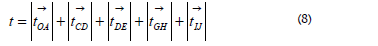
or t = OA + CD + DE + GH + IJ; which is also equal to BC + CD + FG +HI + KL. Regarding τ, we will in Figure. 3 find the current τ - value by adding the abscissas of the red arrows up to the relevant position. Now, indicating a generic notation, we write this as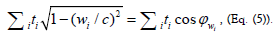For x/c we have to distinguish between the final ‘spatial positions’ 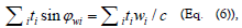and the total distance travelled,

As seen, we restart the process at any instant with change of velocity. The new origin will be defined as the time vector of the clock, being permanently located at the relevant position. Unless also the previous process had w = 0, this requires an update; creating a ‘gap’ in the graph. Giving a more logical approach, this also better illustrates simultaneity of events at different locations; cf. Sec. 4 below.

After a restart, the future process will depend on the new w-value, plus the (t, x) parameters at the update; but not on x, t and τ of the past. This corresponds to the so-called Markov property (‘lack of memory’) in stochastic processes; e.g. [6]. Thus, we may see this event chain as a kind of a Markov process, with the current w-value corresponding to its state.

3.2 Extension to three space coordinates: In the approach, described so far, there is a single space coordinate, x, only. We could, however, introduce three space coordinates (x,y,z) with corresponding velocity coordinates(w_x,w_y,w_z).

Now consider the case of having a constant velocity; having a velocity vector Starting out from the origin at time 0, it follows that calendar time, t at the position (x, y , z) equals At this instant the spatial distance from the origin of K equals

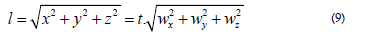
The absolute value of the velocity vector equals Thus, We now apply the results of Sec. 2.1, by just replacing x by l Further is now given by However, if we allow the velocity to change, we must require that the direction of the movement does not alter, in order to maintain a two-dimensional graph.

Observe that there is a kind of analogy between the graphical approach of the present work and Minkowski’s spacetime diagram with three space coordinates, x,y,z, and an imaginary time coordinate, t. The coordinates of his space are (x,y,z,iâ??ct).

As opposed to this, we have transformed the spatial parameters to time, and apply t rather than t as the time coordinate. Minkowski also introduced the spacetime distance, given as in his four-dimensional space, whilst we refer to as the total ‘distance in time’ (from an initiating event) [2].

4. Example: The Twin Paradox

We use the generalized graph of Sec. 3.1 to illustrate variations of the travelling twin case; now considering the entire travel, but applying the same numerical values as an Example 1 of Sec. 2.2.

4.1 The perspective of the earth-based RF, K: The blue graphs of Figure. 4 illustrate the total journey of the travelling twin, in the perspective of the earth’s RF, K. As also seen in Figure. 2a) the travelling twin’s travel to the star is described by OB, at an angle where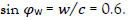

Figure 4:Event graphs of the twins in the perspective of the earth-based RF, K. The blue graphs describe the travelling twin’s journey. The red line, OA follows the earthbound twin, having x/c ≡ 0..

At event, B, having there is an abrupt change in velocity; and a rocket of speed -w starts the return to the earth. We perform an update, and the return starts from the ‘local event’, D. (As previously pointed out, event B, is ‘equivalent’ to the event D; in the sense that both represent t = 5 and x/c = 3.)

The return travel is given by DE and the blue graphs illustrate the result that by the return to the earth, the returning clock has ‘aged’ a value τ = 4 + 4 = 8 years; while it has elapsed a time t = 5 + 5 = 10 years on K.

The red line, OA illustrates the very simple ‘chain of events’ related to the twin remaining on the earth. He is permanently stationed at the origin of K. So, in his case we have w ≡ 0, and thus, ≡ 0, giving x /c ≡ 0 and t ≡ t, (all r). As just found in the blue graph; by the return to the earth, it has elapsed a time t = 10 years on K, and so the red event graph ends at A where t = t= 10 years. We have also inserted the event D*, as the mid-point of OA. So, this occurs on the earth after 5 years, and for symmetry reasons is simultaneous (relative to K) to the start of his brother’s return. By letting this return start at D (rather than B), the diagram well illustrates the simultaneity of these two events, [7].

4.2 The perspective of the travelling twin KT: Now consider the same two chains of events, but viewed in the perspective of another RF. This new RF is denoted KT, with time, tT and position, xT, and it is moving away from the earth at velocity, w. Therefore, we let the travelling twin and his rocket be located at the origin of this RF on its way to the star. At the arrival to the star, this K_T continues its journey away from the earth at the same speed; as we do not allow RFs to change velocity.

Figure. 5 provides an illustration. Again, the red line refers to the travel of the earthbound twin. He is actually moving along the negative xT axis of KT at velocity -w. The corresponding graph has an angle relative to the r-axis, where So, at the end of the process, when his internal clock reads t = 10 years, (as known from Sec. 4.1), it follows that the parameters on K_T for this event equals x_T /c = -7.5 years and t_T = 12.5 years. Thus, the red line fully describes the total journey of the earthbound twin relative to KT

Figure 5: Event graphs in the perspective of the travelling twin’s RF on his travel to the star..

To follow the travelling twin, we look at the blue lines in Figure. 5. For the first four years he remains at the origin of K_T. When t = 4, (and x_T = 0, t_T = 4) there is an abrupt change in his velocity, and the blue line for illustrates his return. Then he has a velocity w relative to the earth’s RF, K. Further, the speed between K and K_T also equals w. Now applying the rule for adding velocities in special relativity (e.g. Eq. (4.15 of [5]), the returning twin will have the following velocity relative to KT:

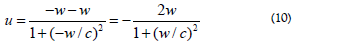
Inserting w/c = 0.6 here, gives u/c = −15/17. So, for the return travel the blue graph has an angle given by −15/17. This fully describes the direction of the blue graph for Further, his journey ends when t = 8 years, (as also known from Sec. 4.1).

We observe that the location on K_T where the two twins are reunited is given by xT /c = -7.5 years, and the clock reading on K_T equals t_T = 12.5 years; which also equals the total length of the blue graph.

4.3 A symmetric approach: Finally, we consider an alternative journey, providing symmetry between the two twins. We apply the same RF, K as in Sec. 4.1, and start out exactly as in that example; Figure. 3 giving an illustration. The travelling twin (blue graph) travels to the star and according to his own clock arrives there after “4 years”. In the present example he remains there until the brother arrives; see DE Figure 6.

Figure 6:Event graphs for the two twins; now reunited at the star.

The other twin (red graph) remains on the earth in 5 years, (OD* ). Then he starts out to the star, with the same velocity as the brother; thus, according to his own clock, arriving there 4 years later. So, according to the stationary clocks on K it has passed 5 years since he left, (DE and D*F). By the reunion, the time on K equals t = 10 years. According to their own clocks, however, the twins agree that it has passed t = 9 years.

Conclusion

The suggested graphical approach provides a useful tool to illustrate the movement of an object with piecewise constant velocity. It gives all relevant time/space parameters, and in particular, this event graph demonstrates how calendar time, t is decomposed into its two components, proper time, τ, and spatial distance (in time units), x/c. Also, the object’s current velocity, w is visualized. The graphs are, for instance, useful for investigating ‘parallel processes’; here exemplified by applying variants of the twin paradox. These examples illustrate both the effect of different ‘perspectives’, (i.e. choices of reference frame), and also different strategies for the reunion of the twins. It thereby supports the comprehension of the phenomenon under investigation

References

1. Epstein LC, Francke D. Book-Review-Relativity Visualized. J. Br. Astron. Assoc, 95(2) 1985; 95:87.

   [Googlescholar]

2. Hokstad P. A graph for describing events in TSR. 2020.

   [Googlescholar]

3. Debs TA, Redhead ML. The twin ‘‘paradox’’and the conventionality of simultaneity. Am. J. Phys. 1996; 64(4):384-92.

   [Googlescholar] [Crossref]

4. Shuler Jr RL. The twins clock paradox history and perspectives. J. mod. Phys.2014.

   [Googlescholar] [Crossref]

5. Mermin ND. It's about time: understanding Einstein's relativity. Princet. Univ. Press. 2006.

   [Googlescholar] [Crossref]

6. Ross SM. Stochastic processes. John Wiley Sons. 1995.

   [Googlescholar]

7. Hokstad, Per, “The Choice of Reference Frame to Determine Time Duration and Simultaneity in Special Relativity”, J Mod App Phy. Vol 6 No 1 March 2023.

   [Googlescholar] [Crossref]