Analytical solution of the steady Navier-Stokes equation for a fluid entrained by a rotating disk of finite radius using the apparatus of tunnel mathematics.

Received: 25-Mar-2022, Manuscript No. Puljpam-22-4578; Editor assigned: 04-Apr-2022, Pre QC No. Puljpam-22-4578(PQ); Accepted Date: Jun 29, 2022; Reviewed: 16-May-2022 QC No. Puljpam-22-4578(Q); Revised: 13-Jun-2022, Manuscript No. Puljpam-22-4578(R); Published: 01-Jul-2022, DOI: 10.37532/2752-8081.22.6.4.1-5

Citation: Shvydkyi OG. Analytical solution of the steady Navier-stokes equation for a fluid entrained by a rotating disk of finite radius using the apparatus of tunnel mathematics. J Pure Appl Math 2022;6(4):1-5

This open-access article is distributed under the terms of the Creative Commons Attribution Non-Commercial License (CC BY-NC) (http://creativecommons.org/licenses/by-nc/4.0/), which permits reuse, distribution and reproduction of the article, provided that the original work is properly cited and the reuse is restricted to noncommercial purposes. For commercial reuse, contact reprints@pulsus.com

Abstract

As is known, if the nonlinear terms in the Navier-Stokes equations for a viscous fluid do not vanish identically then the solution of these equations presents great difficulties, and exact solutions can be obtained only in a very small number of cases. Concerning unsteady Navier-Stokes equation, T. Tao in his article showed that it can have solutions which turn out infinite during finite time (blowup solutions).[1] And if even finite solutions exist they are presented in view of infinite series, that is inconvenient for use in practice. That`s why it is reasonable to seek solutions of steady Navier-Stokes equation in view of elementary functions. Such possibility the equations of analyticity of functions of the spatial complex variable (shortly, the equations of tunnel mathematics) represent since all vector fields, including those obeying the Navier-Stokes equation, satisfy to them. The Navier-Stokes equations themselves are then applied for verification of obtained solutions and calculation the pressure.

Introduction

The exact solution of the problem indicated in the title of the article for an infinite disk is given in the manual on theoretical physics of Landau and Lifshitz (the problem was formulated by Karman) [1]. There this problem was reduced to solving a system of second-order ordinary differential equations which was obtained by numerical methods using a computer [2]. The results of this solution are shown in Figure 1.

Figure 1: Solution of the problem for an infinite disk using numerical methods.

The solution of a similar problem for an infinite disk in the manual of Landau and Lifshitz.

In Figure 1 the function F corresponds to the radial velocity vr, the function G to the circular velocity vφ and the function H to the projection of the velocity vz.

In this case, the disk is located in the plane z = 0 of cylindrical coordinates and rotates around the z axis with a constant angular velocity Ω. The liquid is considered from the side of the disk where z > 0. The boundary conditions for the problem are as follows:

Solution of the problem for a disk of finite radius using the apparatus of tunnel mathematics.

This article provides a solution to a more realistic physical problem when a rotating disk has a finite radius (relatively equal to one). The solution applies only to the volume of the fluid enclosed in a cylinder of approximately unit radius of height z1 (whereг z1 is the height at which the fluid moves in the horizontal mainly radial direction on Figure 2).

Figure 2: Fluid streamlines in one of the planes parallel to the z axis.

The solution implies obtaining analytical expressions (formulas) for three components of velocity and pressure in cylindrical coordinates. Numerical methods are not applicable. The formulas for the velocity components are derived from the relations of tunnel mathematics since the latters are satisfied by all vector fields (including those obeying the Navier- Stokes equations). In this case unnecessary solutions are inevitably obtained and must be cut off by means of a physical analysis of the task at hand. The Navier-Stokes equation is then used for verification of obtained solutions and calculation the pressure.

Just as for an infinite disk the solution of the problem for a fluid entrained by a rotating disk of finite radius will be symmetric with respect to the φ coordinate. Figure 2 schematically shows fluid streamlines in one of the planes parallel to the z axis.

Tunnel mathematics equations are applied to the components of the vector velocity field in Cartesian coordinate system. They look like this [3]:

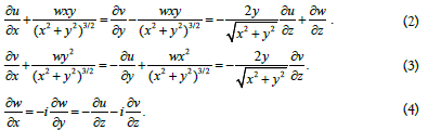
The components of the velocity field in expressions (2-4) are set as follows:

Moreover, the functions u, v, w are components of the function of the spatial complex variable:

As usual the fluid is considered as incompressible:

Taking into account (7) we obtain from equations (2-4):

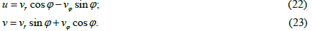
The function w is an analytic function of the variables x and y and, therefore, a harmonic function on the xy plane. So, we can impose:

Any vector fields including those obeying the Navier-Stokes equations satisfy relations (2-4).

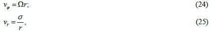
Taking into account the symmetry in the φ coordinate the Navier-Stokes equations in cylindrical coordinates take the following form:

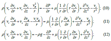
where g is the gravitational acceleration;

P – pressure in fluid;

μ - coefficient of dynamic viscosity;

ρ - fluid density.

Due to the fact that the Laplacian of the analytic function w is equal to zero the equations of tunnel mathematics describe a fluid that moves along the z axis without internal friction, i.e., as an ideal fluid (this is a feature of this method). Taking this into account we can obtain the following form of the function w from equations (5), (9) and (12):

To comply with the dimension expression (13) must be written in the following form:

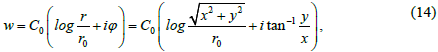
where [С0] = m/s, [r0] = m; we can impose r0 = 1 m.

We find after differentiating (14):

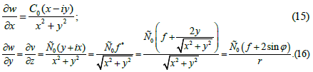
Expression (16) uses the following relations of tunnel mathematics for the operator f and its conjugate operator f* [3]:

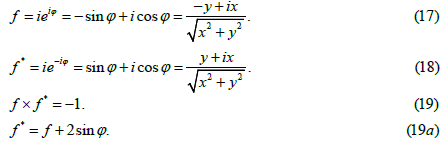
Special attention should be paid to the operator f since the factor at it will be used to reconstruct the spatial coordinate z in the equations on the plane (that corresponds to the relation (6)). We can see from equation (16) that this factor is 1/r (we omit term depending on φ).

Generally speaking, the complex function w must be selected in such a way that its real part meets to the picture of occurring physical phenomena (i. e. to the projection Vz of the velocity field in Figure 2), and the integrating of relations (2) and (3) does not generate integrals that could not be solved in quadratures.

The form of the real part of the function w according to expression (14) is shown in Figure 3.

Figure 3: The graph of the real part of the function w (C0 = 0.05 m/s).

It can be seen from the graph shown in Figure 3 that the radius of the rotating disk should be equal to one (relatively). For r > 1 the fluid streamlines are already rising.

This form of the real part of the function w is inapplicable in the vicinity of the point r = 0 since the graph goes to infinity.

Transforming relations (2) and (3) to cylindrical coordinates and taking into account expressions (8) and (9) we obtain:

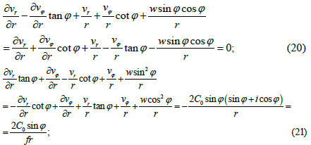
When deriving equations (20) and (21) the well-known formulas were used for the transition from Cartesian velocity projections to cylindrical ones:

Since in the region under consideration (Figure 2) the liquid moves horizontally (mainly radially) when solving equations (20) and (21) we can put w = 0. In equation (21) we work with the real part of the derivative By integrating these equations under such conditions we obtain two solutions for each of the projections of the velocity v_r и v_φ. The solutions that meet to the physical picture of the phenomena of this problem (particularly the boundary conditions (1)) are as follows:

Where σ is a constant of integration.

Expression (25) holds since the solution hasn`t have a dependence on φ, and we work with the assumption (9). Expression (25) is true for r > 1, however, it doesn`t work for r → 0 (it tends to infinity). That`s why it need a correction.

Extension of solutions on a plane into space

To extend solutions (24) and (25) into space we use the factor at the operator f in equation (21):

Where Ф(r, z) is a function of coordinates r and z.

The specific form of the function Ф(r, z) for the projections of the velocity vr and vφ is determined from the integral relations representing the corresponding mass fluxes of fluid through the surfaces of the cylinder covering the region in question (Figure 2).

For radial velocity

So, for the projection r v the following integral relation is used:

Where the integral on the left-hand side represents the mass flux entering through the upper end of the cylinder and the integral on the righthand side represents the mass flux that is scattered through the side surface of the cylinder.

Taking into account equalities (5), (13) and (25), we can write the integral relation (27) in following manner:

Where constants omitted.

Accordingly (26), the presence of the factor in the right-hand side of (28) is sufficient for building of spatial formula. In order to the integral in the right-hand side of (28) doesn’t depend of changing the variable of integration z by r, both variables r and z should enter in the expression for radial velocity r v symmetrically. Then formula (25) can be extended into space as follows:

Where the range of r is (0; 1]; the range of z is (0; z1].

Constants С and С1 are introduced into formula (29) for dimensional compliance. Moreover [С] = m×s, this constant is related to the viscosity of the liquid. And [С1] = m2, this constant has the dimension of area; it can be used to adjust the height z1. For simplicity we can put

С = 1 m×s, С1 = 1 m2.

Spatial and plane graphs for the functions r v from formulas (29) and (25) are shown in Figure 4 and 5 respectively.

Figure 4: Spatial graph for formula (29).

Figure 5: Plane graph for formula (25).

These graphs meet to the picture of physical phenomena arising during the rotation of a disk in a liquid for the following reasons. Let us consider from above the motion of a liquid over a disk at rest in a non-inertial frame of reference for a small value of the z coordinate, when the cohesion forces of liquid molecules with the disk surface still have a noticeable value (Figure 6).

Figure 6: Motion of a liquid over a disk at rest in a non-inertial frame of reference for a small value of the z coordinate.

Coriolis forces due to the circular velocity (the prime means movement in a non-inertial frame of reference) will be directed to the origin of frame of reference and thus will prevent the increase in radial velocity under the action of centrifugal forces . At the same time the Coriolis forces due to the radial velocity will contribute to an increase in absolute value of the circular velocity . As a result of such a dynamic picture the radial velocity having reached its maximum will gradually decrease to zero which corresponds to the graphs shown in Figure 4 and 5.

A similar picture for the same reasons will be observed as the z coordinate increases while the r coordinate remains constant. In this case the radial velocity begins to increase due to the weakening of the cohesion forces between the liquid molecules and the disk surface.

This dependence of the radial velocity component vr on the coordinates r and z can also be explained by energy considerations. If we return to the inertial reference system, then the appearance of a new component of velocity (radial) in it requires certain energy expenditures. Since the energy supplied to the disk for its rotation remains unchanged, an increase in the radial component of the velocity vr is possible only due to a decrease in the circular component vφ which in the inertial frame of reference will tend to retain its value. Therefore, the process of extinguishing the radial component vr in both directions, r and z, will inevitably occur in the liquid.

In this regard a natural question arises as to why in the manual of Landau and Lifshitz the radial velocity depends on the coordinate r according to the linear law [2]:

The point is that formula (30) really takes place for small values of the coordinate r. And since for an infinite disk (namely such a model is considered in the manual of Landau and Lifshitz) any value of r in principle can be considered small, then formula (30) has a full right to life. It is of course inapplicable for a disk of finite radius.

Since in the region under consideration in Figure 2 the liquid moves horizontally (mainly radially), then the projection of the particle velocity on the z axis is zero (vz = 0), and therefore Liouville’s theorem on the invariability of the phase volume of a system of particles is satisfied automatically [4]. The fivefold integral 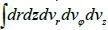is identically equal to zero.

It should also be noted that in accordance with the graphs in Figure 4 and 5 for r > 1 the fluid streamlines must abruptly change the direction of motion so that the vector of the total velocity makes an obtuse angle with the r axis as shown in Figure 2.

For circular velocity

Now let us extend into space the formula (24) for the circular velocity v_ϕ . In this case the following integral relationship applies:

Relation (31) reflects the fact that the mass flux of liquid in the direction of the φ axis through any rectangular section one of the sides of which being the axis of the cylinder in question (Figure 2) remains constant (this impulse never leaves the side surface of the cylinder). Applying formula (24) to expression (31) it is easy to obtain the following relation for reconstructing the z coordinate:

Using relation (32) formula (24) can be extended into space as follows:

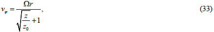
Where 0 z is a normalization factor that is introduced to comply with the dimension.

Figure 7 shows a graph of the dependence of the circular velocity v_ϕ on the z coordinate. It is in principle similar to the corresponding graph in Figure 1 presented in the manual of Landau and Lifshitz.

Figure 7: Graph of the dependence of the circular velocity v_ϕ on the z coordinate.

Verification of the obtained solutions and finding the auxiliary relations

We can at once verify using the true Navier-Stokes equations the solutions (29) and (33) that have been expanded into space by means apparatus of tunnel mathematics. Simplest way to do this is to use equation (11) since it doesn’t contain the pressure P. Substituting solutions (29) and (33), and real part of relation (14), and their corresponding derivative into equation (11) we conclude following important auxiliary relation for z coordinate:

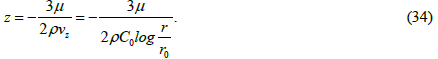
Obtaining relation (34) we imply that magnitude z₀ are small enough (this assumption will be proved below at calculation the friction force acting in a fluid per unit disk surface in a direction perpendicular to its radius). Relation (34) connects the important quantities for fluid, such as coefficient of dynamic viscosity μ, fluid density ρ, and vz which we set manually in this method.

Observing auxiliary relation (34), we see that selecting proper value for C₀ one can regulate magnitude of z coordinate on which the Navier-Stokes equations work. We can conclude that for water (ρ = 1000 kg/m3, μ = 0.001 Pa×s) working coordinate z must be significantly less than 1 meter (z << 1 m).

Also one can verify solutions (29) and (33) using equations (10) and (12). But firstly we must eliminate the pressure P from them. For this purpose, we integrate equations (10) by r, and equations (12) by z. After we subtract equations (12) from equations (10) and, imposing we conclude:

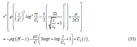
Where H is a depth on which the rotating disc is found; C and C1 are taken from (29); 0 z is taken from (33); C₂(z) is a constant of integration.

If coordinate z has small values (as for water, for example) and constant C₂(z) is appropriately selected, then we can significantly simplify auxiliary relation (35):

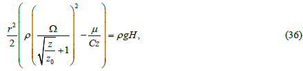
Where Ω is a disc angular velocity.

Calculation of pressure using the Navier-Stokes equations

Using this method, it is still quite difficult to obtain an exact analytical expression for pressure since, for example, equation (12) for projections of velocity on the z axis works only for an ideal fluid.

The approximate formula for the area under consideration in Figure 2 looks like this:

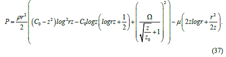
Formula (37) is obtained by integrating equation (10). In this case the corresponding derivatives were calculated using formulas (14), (29) and (33). Generally speaking, we must yet add to right-hand side of formula (37) the hydrostatic pressure ρg(H-z). In Figure 8 and 9 (in Figure 9 the previous graph is slightly rotated around the pressure axis for convenience) graphs corresponding to formula (37) are presented with using the following values of the constants:

The graphs are calculated for water with a density ρ = 1000 кг/м3 and a dynamic viscosity coefficient μ = 0.001 Па×с.

As you can see the graphs shown in Figure 8 and 9 meet to the picture of physical phenomena occurring in the analyzed area in Figure 2. We remind that the radius of the rotating disk is r = 1 m (relatively). Within this area at a fixed coordinate z a diminishing of pressure in the radial direction is observed what corresponds to the movement of the liquid in the horizontal, predominantly radial direction when the disk rotates. As the z coordinate progressively increases the pressure begins to increase what corresponds to the downward fluid flows shown in Figure 2.

Figure 8: Graph corresponding to formula (37)

Figure 9: Previous graph slightly rotated around the pressure axis for convenience.

In the thin boundary layer (very small z) the pressure slightly arises what corresponds the presence of a large tangential-velocity gradient in the boundary layer of fluid, resulting in a large viscous dissipation of energy [2].

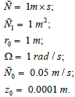
Formula (11) where the pressure is absent due to symmetry along the φ coordinate can be used to calculate the friction force acting in a fluid including per unit disk surface in a direction perpendicular to its radius. Having performed the appropriate calculations, we obtain the following formula for the friction force:

Directing the z coordinate to zero in expression (35) we obtain an expression for the friction force acting on a unit surface of the disk in the direction perpendicular to its radius. To prevent this force from being equal to zero the normalization factor 0 z must be sufficiently small. Therefore, when plotting the graphs in Figure 8 and 9 its value was chosen 0 z = 0.0001 m. The small value of 0 z corresponds to the feature of this method in which the movement of the fluid along the z axis occurs without internal friction.

Conclusion

The solution of the Navier-Stokes equations using the tunnel mathematics apparatus is simple and elegant, and also requires a good mathematical training and a deep physical analysis of the problem. This method does not require a writing of computer programs and can be used for the primary analysis of hydrodynamic problems. The results obtained using this method for a fluid entrained by a disk of finite radius meet to the results of a similar problem in the manual of Landau and Lifshitz solved using numerical methods.

Declaration of Interests

The authors report no conflict of interest.

Data Availability

The data that supports the findings of this study are available within the article.

References

1. Tao T. Finite time blowup for an averaged three-dimensional Navier-Stokes equation. J Am Math Soc. 2016;29(3):601-74.
   Google Scholar                Crossref
2. Landau LD, Lifshitz EM. Fluid Mechanics. Course Theor Phys. 1987;6.
   Crossref
3. Shvydkyi OG. Application of tunnel mathematics for solving the steady Lamé and Navier-Stokes equations.
   Google Scholar                Crossref
4. Landau LD, Lifshitz EM. Mechanics. Course Theor Phys.1983;1.