
Application of tunnel mathematics for solving the steady Lamé and Navier-Stokes equations
Received: 25-Mar-2022, Manuscript No. Puljpam-22-4578; Editor assigned: 04-Apr-2022, Pre QC No. Puljpam-22-4578(PQ); Accepted Date: Jun 28, 2022; Reviewed: 16-May-2022 QC No. Puljpam-22-4578(Q); Revised: 13-Jun-2022, Manuscript No. Puljpam-22-4578(R); Published: 01-Jul-2022, DOI: 10.37532/2752-8081.22.6.3.4-8
Citation: Shvydkyi OG. Application of tunnel mathematics for solving the steady Lam�© and Navier-Stokes equations. J Pure Appl Math 2022;6(3): 4-8.
This open-access article is distributed under the terms of the Creative Commons Attribution Non-Commercial License (CC BY-NC) (http://creativecommons.org/licenses/by-nc/4.0/), which permits reuse, distribution and reproduction of the article, provided that the original work is properly cited and the reuse is restricted to noncommercial purposes. For commercial reuse, contact reprints@pulsus.com
Abstract
The theory of functions of a complex variable is a hybrid of vector algebra and ordinary algebra. It makes it possible to work with vector quantities as with algebraic ones. The modern theory of functions of a complex variable was created by the French mathematician Augustin Cauchy (1789-1857), later it was rapidly developed and found its application in solving various problems of physics in aerodynamics, hydrodynamics, elasticity theory, etc. However, this theory is used exclusively for solving problems on the plane. Therefore, the next natural step is to extend this theory into space, so that we can obtain the solution of physical problems directly in space. The creation of such a theory is associated with some serious problems, for example, the appearance of so-called zero divisors, spatial complex numbers that are not equal to zero but when multiplying for some reason give zero. There is also a Frobenius theorem which prohibits the propagation of complex numbers into a space without abandoning some ordinary algebraic operations (for example, commutative multiplication). In this article an attempt is made to construct a theory of spatial complex functions (shortly, tunnel mathematics) in which zero divisors do not appear and all the usual algebraic operations are preserved. The possibility of applying this theory to some problems of the theory of elasticity and hydrodynamics (the steady Lamé and Navier-Stokes equations) is also considered.
Introduction
Determination of a spatial complex number
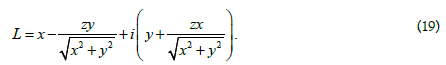
Similar to how a vector is defined in three-dimensional space, we define a spatial complex number as follows:

Where ReL – is a real part of a spatial complex number L, ImL - its imaginary part, FantL - its spatial part.
The spatial complex number L is shown in Figure1.

Figure 1: Spatial complex number L.
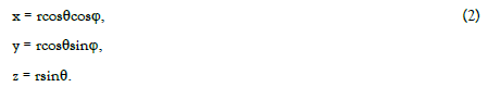
The components of the space vector expressed in terms of its magnitude r as well as the angles φ and θ are defined as follows:
On the other hand, the following obvious equality holds:

Now, if we introduce the operator

Then on the right in formula (3) we obtain the expansion of the space vector with unit modulus along the x, y, z axes. The components of this expansion coincide with the values of the projections in formula (2) at r = 1.
Thus, the simple rotation in the ordinary complex plane xy of the unit vector with the argument φ by the angle θ corresponds to the appearance of a spatial complex number (having a spatial coordinate z). We rotate not in the plane xy but in the plane perpendicular to it (that is not prohibited). Therefore, the angle θ is the angle between the direction of the space vector and its projection onto the xy plane (Figure 1). So the true nature of this spatial theory of complex functions still remains plane but the results obtained on the plane in a certain way can be transferred into space. The spatial axis z, as it were, folds into the xy plane with a hinge at the origin and rotates about the angle φ by 90 degrees counterclockwise. The fact that the spatial theory of complex numbers remains essentially plane has a huge plus when solving spatial problems, we can use all the powerful potential of the plane theory of functions of a complex variable.
So the spatial complex number is given by formula (1) where x, y, z are the real numbers.
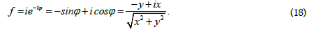
The exponential form of the spatial complex number is:
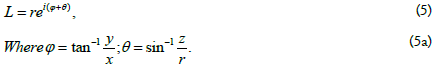
The trigonometric form is as follows:

We define the conjugate spatial complex number as follows:
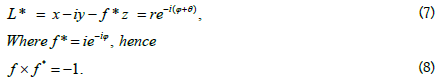
Identical to plane theory, the following relation holds:

Meanwhile the following relationships hold:
Considering that
We can define spatial complex number on a plane as follows:
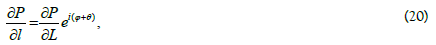
The derivative in the direction l of an arbitrary function of the spatial complex variable P defined by the angles φ and θ is calculated by the formula:
Where L is defined by the formula (1).
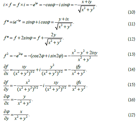
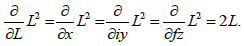
The derivatives in the directions of the x, iy, fz axes are equal to each other and are calculated as in the usual plane theory. So, for example, the derivative of a quadratic function of a spatial complex variable is:
New Cauchy-Riemann conditions
Let us derive conditions similar to the Cauchy-Riemann conditions in the plane theory which are necessary for the spatial function to be analytic. These conditions (let’s call them the New Cauchy-Riemann conditions) as in the plane theory are derived from the requirement that the derivatives of the function of the spatial complex variable in the directions x, iy, fz are equal to each other.
Consider the following spatial complex variable function:

Where functions u, v, w are, generally speaking, complex functions of real variables x, y, z.
In order for the derivatives of the function P(L) in the directions x, iy, fz to be equal to each other the following relations must hold:
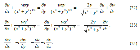
It follows from condition (24) that the derivatives of the complex function w in the directions x and iy are equal, therefore the function w is an analytic function of the variables x and y and, therefore, a harmonic function on the xy plane. This means that the relation holds:
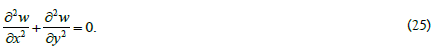
It turns out that the function P(L) has a “harmonic tail”.
Axis z can be called a combine coordinate axis or overaxis. This situation arises because the complex space is built by the intersection of two usual mutually perpendicular complex planes, as shown in Figure 2.

Figure 2: Formation of a complex space by the intersection of two mutually perpendicular ordinary complex planes (axis fz is the overaxis).
Formula (3) based on such model.
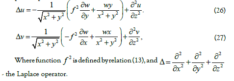
The analysis of relations (22) and (23) leads to the next formula for complete Laplacian of functions u и v:
The analysis of relations (22) - (24) and (13) leads to the next equations for the function P(L) from formula (21):
The relations (24) with condition  leads to the next equation:

Application of the obtained results in the theory of elasticity
The obtained properties of the triplet of functions u, v, w can be immediately applied to the solution of some applied equations, for example, the Lamé (or Navier) equations in the theory of elasticity. As we know, the steady Lamé equations are as follows [1]:
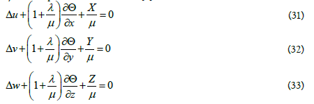
We assume that a triplet of functions u, v, w, which satisfy the New Cauchy-Riemann conditions (22) - (24) and the relations (25) - (30), are displacements along the x, y, z axes respectively for elastic deformation of an isotropic body. In this case naturally the functions u, v, w are measured in meters, i. e.
[u] = [v] = [w] = m.
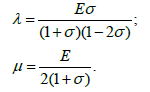
In equations (31)-(33) the coefficients λ and μ are elastic constants characterizing the material (moreover, μ is the shear modulus). These constants are related to Young’s modulus E and Poisson’s ratio σ as follows:
The quantities λ and μ are measured in Pascals, i.e.
[λ ] = [μ ] = Pa
Dimensionless quantity

is the relative volumetric expansion of the deformed body.
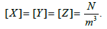
The quantities X, Y, Z are the projections of external volumetric forces applied to the deformable body on the x, y, z axes respectively. The dimensions of these quantities are as follows:
The dimensions of the Laplacian functions are as follows:
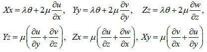
During elastic deformation relative displacements are introduced as follows:
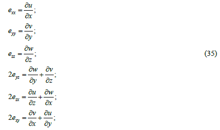
In this case the first subscript near the letter e denotes the axis along which the deformation occurs; the second subscript indicates which axis is perpendicular to the area on which the deformation occurs. The last three formulas define shear displacements.
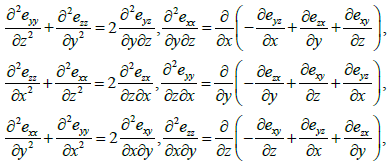
Since the derivatives of the functions u, v, w enter in relations (22) - (24) in a linear manner the relative displacements (35) satisfy (what can be verified by direct substitution) to six Saint-Venant compatibility conditions which as is known are written as [1]:
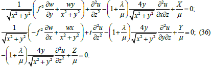
After applying relations (22) - (30) the Lamé equations (31) - (33) take the following form:
The system of equations (36) can be significantly simplified if the second equation is multiplied by ⅈ and added to the first equation:
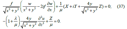
As we see from equation (37) the projections of the external volumetric forces X, Y, and Z are completely determined by the harmonic tail of the function P(L), i.e. by the function w which corresponds to the displacement of the deformed body along the z axis. If this function is set in advance (as we know the harmonic function can represent exclusively the potential and solenoidal (without sources and sinks) field of relative displacements) as well as at least one of the projections of external volumetric forces (for example Z) then the other three unknown functions can be found. The strain tensor components are calculated using the following formulas [1]:
Some integral relations of tunnel mathematics
It`s known that in a plane theory of functions of a complex variable it is always possible to find the value of the analytic function inside a region knowing its values at the boundary of this region. For this aim the Cauchy integral formula is applied:
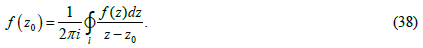
Here f(z) simply denotes a function of a complex variable in the plane.
A similar formula, in which integration is performed over a sphere S of radius R, works for spatial analytical functions:
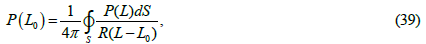
Where sphere area element is defined as follows:

That corresponds to the surface element ndS in mathematical analysis.
Figure 3 explains formulas (39) and (40).

Figure 3: To the derivation of integral relations in complex space.
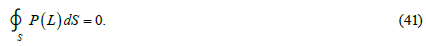
It is of interest to find the flux of a function of the spatial complex variable P(L) through the sphere S and determine the conditions under which it is equal to zero (i. e., determine the conditions under which the source or sink of vector field goes out the boundaries of the sphere S). So consider the integral
The part of used for this purpose Gauss-Ostrogradsky formula has the form:
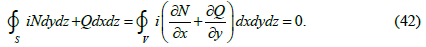
Performing the calculations, we conclude the integral in formula (41):
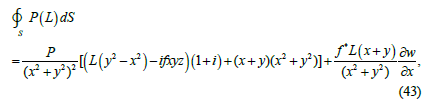
Where f* is defined by formula (11) and L is defined by formula (1).
We see from formula (43) that if the function w is equal to a constant then the flux of the function of the spatial complex variable P(L) through the sphere S is equal to zero only in the trivial case.
Application of the obtained results in hydrodynamics
Using relations (22) - (27) it is possible to integrate the steady Navier-Stokes
equation for an incompressible fluid when its particles are isentropically
moving in circular orbits. This model corresponds to a fluid that moves
between two coaxial cylinders rotating around its axis [2]. The components
of the vector velocity field V of the liquid particles are set as follows: Vx = u;
Vy = v; Vz = w. As is known the condition of incompressibility (solenoidality)
of a liquid is expressed by the equality to zero of the divergence of its vector
velocity field, i.e.,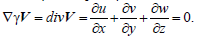
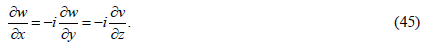
From equations (22) and (23), and assumption  the condition
for the incompressibility of the fluid can be expressed in the following simple
way:
the condition
for the incompressibility of the fluid can be expressed in the following simple
way:

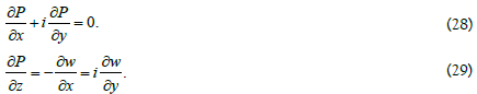
Then relation (24) takes the form:
As you know, the vorticity of the vector velocity field is defined as follows:
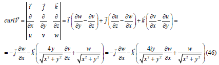
That is the vorticity of the velocity field of liquid particles is completely determined by the harmonic tail of the function of the spatial complex variable P(L), i.e., by the function w in equation (21). Since the function w is harmonic in the xy plane and determines the projections of the particle velocities on the z axis it can describe exclusively the irrotational (potential) and solenoidal (without sources and sinks) field of spatial accelerations of liquid particles out of the xy plane. As a first approximation we require that the vorticity of the vector velocity field defined by expression (46) has no projection onto the y-axis. Thus, we arrive at the following relations:
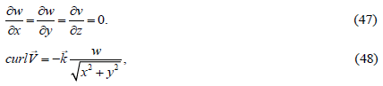
Where the function w is equal to a constant. If this constant is zero, the vorticity disappears. Of course, in this case the vortex motion of the fluid occurs only in the xy plane.
To find the steady Navier-Stokes equation we proceed from Newton’s second law for bulk of fluid in a frame of reference associated with a rotating fluid:
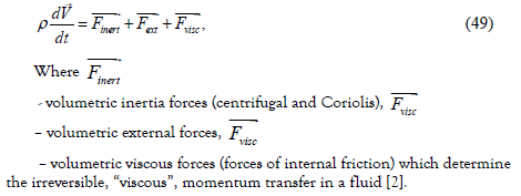
Expressing the volumetric external forces through the gradient of pressure Р, and the volumetric viscous forces - through the Laplacian of the velocity field we have:

Taking the curl operation from both sides of equation (50) and grouping the terms accordingly we get:
Hence it follows that the vorticity of the fluid is provided by the vortex
field of volumetric inertia forces inert  . (more precisely, Coriolis forces since centrifugal forces can be expressed through the gradient of the scalar field).
Expanding in (50) the total time derivative of the fluid velocity field we obtain the well-known Navier-Stokes equation:
Assuming the partial time derivative  equal to zero we obtain the
steady Navier-Stokes equation in projections:
equal to zero we obtain the
steady Navier-Stokes equation in projections:
Where Fx, Fy – the projections of the volumetric inertial forces acting in the ху plane;
gz = g is the projection of the gravitational acceleration onto the axis z which is directed downward;
P – fluid pressure;
μ - now is the coefficient of dynamic viscosity;
ρ - fluid density.
Applying relations (47) to equation (55) we immediately find an expression for that part of the pressure in the liquid which is determined by the increment of the coordinate z:

Where С (х, у) – the constant of integration. Thus, Pz is the usual static pressure of the fluid in the gravity field.
We assume that the field of volumetric Coriolis forces  completely
belongs to the xy plane. Using the apparatus of tunnel mathematics, we can
easily obtain an expression for the curl of this field.
completely
belongs to the xy plane. Using the apparatus of tunnel mathematics, we can
easily obtain an expression for the curl of this field.
We multiply equation (54) by ⅈ, equation (55) by f, after which we add up equations (53), (54) and (55) term-by-term. Applying relations (22), (23), (29) and (30) we obtain:
Where Finert and ∇P are spatial complex functions of volumetric forces of inertia and external forces of the function type (21).
Taking the curl operation from both sides of equation (57) we get:
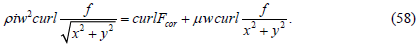
Taking into account the value of the operator f from formula (18) we find the vorticities of the quantities in (58) as the curls of ordinary vector fields. After performing the calculations, we get:
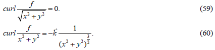
Substituting the values (59) and (60) in (58) we find the expression for the vorticity of the field of volumetric Coriolis forces:
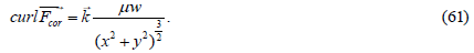
It follows from expression (61) that the curl of the field of volumetric Coriolis forces depends on the dynamic viscosity of the liquid and does not depend on its density; it also rapidly decreases to zero with increasing radius of the trajectory of liquid particles (~ r−3 ). (In this section the letter r denotes the radius of the particle trajectory in the ху plane.)
By integrating relations (22) and (23) subject to conditions (44) and (47) we can find the projections of the velocity field of the liquid V on the axis х и у:
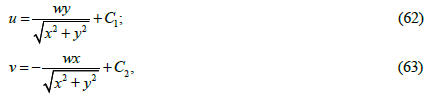
Where C1, C2 are integration constants, which are set equal to zero.
It is easy to see that the projections of the velocity field u and v from expressions (62) and (63) correspond to circular trajectories of liquid particles in the xy plane which move clockwise (that corresponds to the sign of the curl of the velocity field in formula (48)) with constant circular velocity equal to w. It is easy to check by direct calculation that the value of the curl of a given velocity field also corresponds to formula (48). Such field can belong to liquid particles that move between two coaxial cylinders rotating around their axis [2] provided that the distance between the cylinder walls is small enough
(R2 − R1 = h = R1 ).
A simple formula follows from the expressions (62) and (63):
u2 + v2 = w2 (64)
We solve the steady Navier-Stokes equations (53) and (54) in an immobile frame of reference, i.e., without taking into account the forces of inertia Fx and Fy (solutions in a moving frame of reference can be easy obtained according to well-known rules). Applying relations (22) - (27), (44), (47) to them as well as the newly obtained relations (62) and (63) we obtain the following equations for determining the pressure in a liquid:
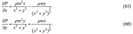
If we add to equation (65) the expression 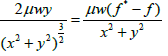 tending to zero with growing distance from the z axis (equality corresponds
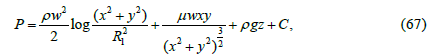
to the formula (12)) then the pressure P can be expressed analytically:
tending to zero with growing distance from the z axis (equality corresponds
to the formula (12)) then the pressure P can be expressed analytically:
It was taken into account when integrating that if the distance between
the walls of the cylinders is small enough then the value  remains
practically constant.
remains
practically constant.
Figure 4 shows a graph of water pressure between rotating coaxial cylinders that corresponds to formula (67) when the constant C and the z coordinate are equal to zero and the value of the circular velocity w is 1 m/s. The radius of the smaller cylinder R1 is taken as 0.5 m. The water pressure in the direction of the larger cylinder increases along the generatrix of the funnel in the figure. The presence of the second term on the right side of formula (67) practically does not affect the graph due to the smallness of the dynamic viscosity coefficient of water (μ = 0.001 Pa×s) in comparison with its density (ρ = 1000 kg/m3).

Figure 4: Water pressure between rotating coaxial cylinders provided that the distance between the cylinder walls is small enough.
Since formula (67) is used to calculate the fluid pressure between rotating coaxial cylinders provided that the distance between the cylinder walls is small enough
(R2 − R1 = h = R1 ).
this formula can be used to calculate the fluid pressure for the same model when the distance between the walls of the cylinders becomes a finite value. To do this we need to know how the circular velocity w which was assumed to be constant in formula (67) depends on the coordinates on the plane. For a model of two rotating coaxial cylinders the circular velocity w depends on the polar coordinates as follows [2]:

Where a and b are the constants.
Taking the differential from expression (67) and considering all quantities to be constant, except for w, and omitting the second term depending on the polar angle φ, and also taking the differential from expression (68) we get:
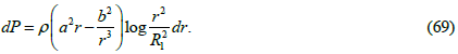
After integrating of expression (69) by parts we obtain a formula for the fluid pressure between rotating coaxial cylinders when the distance between the cylinder walls becomes a finite value:
Figure 5 shows a graph of water pressure between rotating coaxial cylinders corresponding to formula (70) when the constant C and coordinate z are equal to zero and the constants a and b are equal to unity. The radius of the smaller cylinder R1 is taken as 0.5 m. The value of R1 must be outside the area of a sharp pressure dropping.

Figure 5: Water pressure between rotating coaxial cylinders when the distance between their walls becomes a finite value.
Conclusion
In this article the conditions for the analyticity of the spatial function of a complex variable (essential relations of tunnel mathematics) were obtained and used for solving some steady equations of the theory of elasticity and hydrodynamics.
Data Availability
The data that supports the findings of this study are available within the article.
Declaration of Interests
The authors report no conflict of interest.
REFERENCES
- Muskhelishvili NI. Some Basic Problems on the Mathematical Theory of Elasticity: Fundamental Equations. Plane Theory Elast Torsion Bend. 1975;1963:347.
Google Scholar Crossref - Landau LD, Lifshitz EM. Fluid mechanics. Course Theor Phys. 1987;6.
Google Scholar Crossref