Choice of Reference Frame to Determine Time Duration and Simultaneity in Special Relativity
Received: 10-Feb-2023, Manuscript No. puljmap-23-6151; Editor assigned: 12-Feb-2023, Pre QC No. puljmap-23-6151(PQ); Accepted Date: Feb 24, 2023; Reviewed: 14-Feb-2023 QC No. puljmap-23-6151(Q); Revised: 16-Feb-2023, Manuscript No. puljmap-23-6151(R); Published: 28-Feb-2023, DOI: 10.37532.2022.6.1.1-4
Citation: Hokstad P. Choice of reference frame to determine time duration and simultaneity in special relativity. J Mod Appl Phys. 2023; 6(1):1- 4
This open-access article is distributed under the terms of the Creative Commons Attribution Non-Commercial License (CC BY-NC) (http://creativecommons.org/licenses/by-nc/4.0/), which permits reuse, distribution and reproduction of the article, provided that the original work is properly cited and the reuse is restricted to noncommercial purposes. For commercial reuse, contact reprints@pulsus.com
Abstract
Rather than adopting the conventionality of simultaneity, we discuss the possible identification of a ‘correct’ Reference Frame for analyzing time duration and simultaneity of phenomena. Three standards. Examples are reviewed to illustrate the approach. The discussion includes the use of the concepts, time vector and event graph.
Key Words
Simultaneity, Symmetry, Time vector, Event graph, Travelling Twin, µ-mesons.
Introduction
n the theory of special relativity moving reference frames provide different results both for the duration of a chain of events and for the simultaneity of events. Many authors discuss the relativity of simultaneity [1]. Which argues for a version of the conventionality of simultaneity: There will be a time interval of events, all being simultaneous to a (distant) event; which of these to choose is rather a matter of convention. In contrast, we here argued that one should properly specify the phenomenon under investigation; and thereby identify one ‘correct’ perspective; a specific Reference Frame (RF) from which the events should be considered. This leads to one ‘canonical’ result for the duration and simultaneity of events. Our discussion is based on three standard examples: The Travelling Twin (TT); two spacecrafts moving relative to each other in outer space, and the case of the μ-mesons.
Background
First some basic terminology, assumptions and tools are provided.
Notation
We start out from a RF denoted K, which for simplicity has just one space coordinate (X). The RF has synchronized, stationary clocks located at virtually any position. Further, there is an object moving at velocity, w relative to K along the x-axis. The object starts out from the origin of K when the clock at this position on K reads 0. Further, (we imagine that) this moving object brings with it a clock, and when the object passes the origin at time 0, this clock is synchronized with the clock on K at this position. Three fundamental parameters are related to the movement of this object.
First
τ =Clock reading of the clock following the moving object. We would say that this is the ‘internal time’ of the object/event, but usually, this is referred to as the ‘proper time’.
This proper time, τ is independent of which RF we choose as the basis for our observations. Further, we have two parameters (t, x), which specify events on the chosen RF, K.
x=Position of the moving object relative to K, (when the passing clock reads τ).
t=Clock reading of the clock permanently located at position x on K, when the moving clock reads τ; (this t is usually referred to as ‘calendar time’).
Further, we have w=x/ t, i.e. the velocity of the object relative to the RF, K.
c=speed of light, then according to the so-called time dilation in special relativity [2], we have the fundamental relation
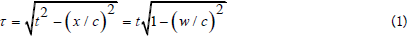
Now, we proceed to introduce the time vector of an event (t, x), cf [3].
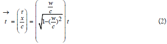
Note that the absolute value of this vector equals

Thus, the time vector comprises the information of all the fundamental parameters of an event. Note that the three parameters τ, t and x/c all represent time. In particular, x/c equals the time required for light to traverse the distance x (from the origin to the location of the event). (According to eq. (3) it could seem rather sensible to denote t for the ‘total time’; as it is split into two components of time).
Event Graph
We will illustrate the discussion with an event graph. This will provide a graphical representation of the difference in the time vector from a certain initiating event [4].
Thus, a graph illustrates a chain of events, say, a clock moving at constant velocity relative to a specific RF, K. Figure 1 illustrates the ‘movements’ in space-time of three relevant clocks in the well-known Travelling Twin (TT) example. The graphs are relative to the earth’s RF, K; considering just the period from the departure from the earth until the TT’s arrival at the star. In Figure 1 the ‘distance’ to the star equals OC; the event vector OB represents the travel of the TT. The vector OA is the corresponding change in the time vector of the earthbound twin, and CD represents the (imagined) clock permanently located at the star. For both these clocks there is (of course) no change in x/c. All the vectors OA, OB and CD have the same length; i.e. the time required for the TT to reach the star (according to K).

Figure 1: Following the three relevant clocks of the TT case; (travel to the star). The perspective of the earth
Choosing the Right Reference Frame
Simultaneity within a single inertial Reference Frame (RF), K is verified by synchronized clocks [2, 5]. For events having the same clock reading, t on this RF we have simultaneity ‘in the perspective of K’. Clocks on different RFs will not agree on the simultaneity, and this has led to the concept of relativity of simultaneity (and conventionality of simultaneity). However, we will claim that even if there is an infinite number of RFs to describe the chain of events, there is (typically) one that stands out as the appropriate one. This RF gives the ‘correct’ result both for durations and simultaneity of events. We now illustrate this statement on time duration and simultaneity in the theory of special relativity by looking at three standard examples.
Example 1: The travelling twin
The travelling twin paradox is discussed [1, 6]. We apply a standard
numerical example [2]. The Travelling Twin (TT) leaves the earth in a
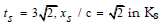
rocket of velocity, v=0.6 c (with respect to the earth). This gives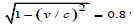 He travels to a ‘star’ at a distance of 3 light
years from the earth. Thus, this distance equals x=3 c. The earth’s RF
has a clock located at the star, and by the arrival of the TT, this clock
will read
He travels to a ‘star’ at a distance of 3 light
years from the earth. Thus, this distance equals x=3 c. The earth’s RF
has a clock located at the star, and by the arrival of the TT, this clock
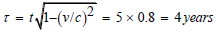
will read  At this instant the
travelling twin’s clock will according to special relativity read
At this instant the
travelling twin’s clock will according to special relativity read
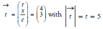
In summary, the arrival of the rocket to the star represents the following event (in the earth’s RF).
 corresponding to the time
vector
corresponding to the time
vector
As discussed above, Figure 1 illustrates the travel to the star. In Figure 2 we now illustrate the total travel, using the above numerical values. This includes an abrupt change in the velocity of the TT; requiring a new initiating point; actually, we should rather include a second space ship moving towards the earth with velocity –v1. The returning spaceship must be given the clock reading, t=5; thus the ‘retuning TT’ adopts the time vector of the local clock at the star. The returning TT (or at least the new calibrated clock) is illustrated by the blue line DF. Thus, the TT’s travel is actually given as two distinct travels; OB + DF. The total length of these two travels equals the change in the clock rate of the earthbound twin (i.e. 10 years). The red line OE represents the event graph for the earthbound twin.

Figure 2: Event graphs of the twins in the perspective of the earth-based RF, K. The blue graphs describe the travelling twin’s journey. The red line, OE follows the earthbound twin, having x/c ≡ 0
It remains to argue why this RF (of the earth) must be the correct one here. Actually, both phenomena (series of events for the two twins) take place relative to this RF. In particular, when the TT returns to the earth the clock of the TT will read 8 years and that of the earthbound twin will read 10 years, as predicted by the perspective given in Figure 2. Observers moving relative to the phenomenon will obtain different results. Also see discussion in Example 2 below. When the RF is specified, the correct results concerning time durations and simultaneity follow. In particular, we could ask which event on the earth is simultaneous with the arrival of the TT at the star.
Now the answer is that this arrival is simultaneous with the earthbound twin’s clock reading t=5 years (identical to the clock reading at the star). The symmetry of the travel to and from the star demonstrated in Figure 2 supports this
Example 2: two space crafts
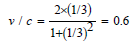
Now consider two spacecrafts in outer space. They start out simultaneously in opposite directions from the same position. Our intention is that the experiment shall be completely symmetric with respect to the two spacecrafts. So as our RF we now introduce KS with its origin at their common starting point; and the spacecrafts move relative to this RF at velocities w and -w, respectively. Further, we choose w=c/3, which means using the standard formula for adding velocities in special relativity that the relative velocity between the two spacecrafts is given by
This is in fact the same velocity as that of the TT relative to the earthbound twin, (see Example 1), giving an obvious link to that example. To further link these two cases, we let KS move relative to K at speed w. Thus, one spacecraft is stationary with respect to K, and the other has speed v relative to K (in complete analogy with the two twins).
When τ = 4 years we have (since τ is independent of the RF), that the spacecraft moving to the right has travelled the distance to the star. As its speed relative to KS equals w=c/3, simple calculations give that this corresponds to the event
This is now illustrated by the event graphs in Figure 3. The line OB
represents the spacecraft moving the distance from the origin to the
star (relative to K), and OC the travel of the other spacecraft. At this
point the two spacecrafts start on their travel to reunite. In order to
maintain a complete symmetry, they both reverse their velocity, and
doing so, we define new initiating points: their clocks are calibrated
to read  Thus, the line DF represents the travel of the first
spacecraft back to the origin of KS, and similarly for the other one
(sees the blue lines). The red line OE represents events describing the
origin of KS. Trying now to ignore the various technicalities, Figure 3 can in principle be seen as the event graph of two phenomena, both
the TT and the two spacecrafts. But as these graphs obviously fail to
give a proper illustration of the TT case, (definitely giving wrong
results for the clock reading when the twins reunite), it very well
describes the symmetry of the spacecraft example. In particular it
gives the same ‘age’ as they reunite. This symmetry also fits the
discussion of simultaneity at the turning of the spacecrafts. Here we
have simultaneity when the clocks of KS read
Thus, the line DF represents the travel of the first
spacecraft back to the origin of KS, and similarly for the other one
(sees the blue lines). The red line OE represents events describing the
origin of KS. Trying now to ignore the various technicalities, Figure 3 can in principle be seen as the event graph of two phenomena, both
the TT and the two spacecrafts. But as these graphs obviously fail to
give a proper illustration of the TT case, (definitely giving wrong
results for the clock reading when the twins reunite), it very well
describes the symmetry of the spacecraft example. In particular it
gives the same ‘age’ as they reunite. This symmetry also fits the
discussion of simultaneity at the turning of the spacecrafts. Here we
have simultaneity when the clocks of KS read  and the
internal clocks of the spacecrafts read τ=4 years. So, by choosing the
correct RF for the actual phenomenon under investigation, we can
actually identify one correct answer.
and the
internal clocks of the spacecrafts read τ=4 years. So, by choosing the
correct RF for the actual phenomenon under investigation, we can
actually identify one correct answer.

Figure 3: Event graphs for the two rockets; in the perspective of the symmetric RF, KS
Example 3: The case of the μ-mesons
As a final case, we discuss the example of the μ-mesons [2]. The μ- mesons are produced by cosmic rays in the upper atmosphere. When 'at rest' they have a lifetime of about 2 microseconds, so if their internal clocks ran at a rate independent of their speed, even if they travelled at the speed of light about half of them would be gone after they had travelled 2.000 feet. Yet about half of the μ-mesons produced in the upper atmosphere (about 100.000 feet up) manage to make it all the way down to the ground. This is because they travel at speed so close to the speed of light that the slowing down factor equals 1/50, and they can survive for 50 times as long as they can when being stationary.
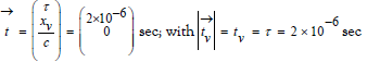
This phenomenon is easily described by the Lorentz transformation. We have two RFs; that of the earth, K, and that of the μ-mesons, named Kv (with parameters (tv, xv)). We will refer to the creation of the μ-mesons in the upper atmosphere as the initiating event A. At this event, x=xv=0 and t=tv=0. Further, we refer to the arrival at the ground as event B. At this event xv=0 and tv=2∙10-6 sec. Thus, in Kv we then have τ=tv=2∙10-6 sec, and we get the time vector
Further, this event B has the same τ- value in the RF K of the earth, and the μ-mesons have then gone the distance x = 105 feet in K, giving x/c ≈ 10-4 sec. Thus, the time vector of event B, as specified in K equals
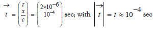
So, these two time vectors verify the given observations, stating that
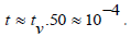
In summary, the given observations are in full agreement with the theory. It is an experimental fact that the (imagined) clock following the μ-mesons goes slower by a factor 50, when it is compared with two clocks, being stationary relative to the earth. But, how shall we interpret/refer to this? It is somewhat surprising that formulates the findings as: "The atomic particles can go much further because their internal clocks that govern when they decay are running much more slowly in the frame in which they rush along at speed close to c [2]. This is a real effect, and it plays a crucial role in the operation of such particles accelerators”.
However, rather than referring to this as a real effect, I suggest it should be referred to as an observational effect; caused by the observer (at K) moving relative to the occurring phenomenon (taking place on Kv).Similarly, regarding use of the concept internal clocks (of the atomic particles): Actually, if the observer (the observing clock) is at rest with respect to the phenomenon, then he will find that the average ‘lifetime’ of the μ-mesons equals 2 microseconds. So, it is rather this value we should consider to express the ‘internal clock’ of the μ-mesons. Passing observers - at various speeds, v will make ‘all kind’ of observations, (depending on v). And an 'inner clock' should hardly be affected by passing observers. So, we should rather see= 2×10⁻⁶ to represents the ‘true’ lifetime of the μ-mesons also in the present experiment [7].
So, in my view, this case exemplifies the argument that the correct RF to describe the phenomenon is the one which follows the event. It is the phenomenon itself and not the observer should have priority.
Summary and Conclusions
The above discussions suggest that it does exist one RF, being best suited to describe a phenomenon; and thus, providing time durations and simultaneity of events. We now outline the following rules for specifying the framework of the analysis.
1. We choose an RF that follows the phenomenon as closely as possible; in particular the observing RF shall not move relative to the to the process.
2.The RF shall secure that any inherent (or chosen) symmetry of the situation is accounted for; (but not any ‘unwanted’symmetry).
3.When an initiating event (or a set of events) is defined, the‘internal’ clocks of these events are calibrated with the localclock on the RF.
4.We stick to the chosen RF throughout the experiment; i.e. wedo not change RF during the course of events.
5.When there is a change in the velocity of one or more movingobject/event involved, we specify a new initiating event andupdate clocks accordingly.
When we discuss simultaneity, we assume here that the chains of events being involved start out from one single initiating event. The argumentation is based on investigating the logical implications of the initial conditions and the rules of special relativity (the Lorentz transformation). This might include bringing the supposed ‘simultaneous’ clocks together again, and derive their readings at this instant, (representing ‘true’ simultaneity).
References
- Debs TA, Redhead ML. The twin ‘‘paradox’’and the conventionality of simultaneity. Am. J. Phys., 1996; 64(4):384-92.
- Hodgson TR. It's About Time: Understanding Einstein's Relativity. Mathematics teacher. 2006; 100(2):158-9.
- Hokstad P. A new concept for simultaneity in TSR. 2018
- Hokstad P. A graph for describing events in TSR ., 2023.
- Giulini D. Special Relativity: A First Encounter: 100 years since Einstein: 100 years since Einstein. OUP Oxford.
- Shuler Jr RL. The twins clock paradox history and perspectives. Journal of modern Physics. 2014.
- Dehghani P, Frank M. Reconciling collider signals, dark matter, and the muon anomalous magnetic moment in the supersymmetric. ArXiv preprint. 2023.