Coupled systems of boundary value problems for nonlinear fractional differential equations

Received: 05-Jun-2018 Accepted Date: Jun 25, 2018; Published: 29-Jun-2018, DOI: 10.37532/2752-8081.18.2.8

Citation: Shah K. Coupled systems of boundary value problems for nonlinear fractional differential equations. J Pur Appl Math. 2018;2(2):14-17.

This open-access article is distributed under the terms of the Creative Commons Attribution Non-Commercial License (CC BY-NC) (http://creativecommons.org/licenses/by-nc/4.0/), which permits reuse, distribution and reproduction of the article, provided that the original work is properly cited and the reuse is restricted to noncommercial purposes. For commercial reuse, contact reprints@pulsus.com

Abstract

In this article, we study coupled systems of boundary value problems for fractional order differential equations. We use the idea of the Generalized matric space to develop necessary and sufficient conditions for uniqueness of positive solutions of the system. We also obtain sufficient conditions for existence of at least one solution via nonlinear differentiation of Leray Schauder type. We include an example to illustrate our main results.

Keywords

Coupled system; Fractional differential equations; Riemann-liouville boundary conditions; Existence; Uniqueness results

Recently the theory on existence and uniqueness of solutions of fractional differential equations have attracted much attentions and a large number of research articles on the solvability of nonlinear fractional differential equations are available. We refer to [1-4] and the references therein for some of the recent development in the theory. On the other hand, coupled systems of boundary value problems for non linear fractional differential equations are not well studied and only few results can be found dealing with existence and uniqueness of solutions [5-8]. Su [5] developed sufficient conditions for existence of solutions to the following coupled systems of two point boundary value problems

D^α u(t) = f (t,v(t),Dμ v(t)), D^β u(t) = g(t,u(t), Dν u(t)), 0 < t <1, u(0) = u(1) = v(0) = v(1) = 0,

where 1<α ,β ≤ 2,μ,ν satisfies α −μ and β −ν ≥1 and f , g :[0,1]× R× R→ R are continuous and Dis the standard Rieman- Liouville derivative. Wang et al. [8] obtained sufficient conditions for existence and uniqueness of positive solutions to the following coupled systems of nonlinear three-point boundary values problems

D^α u(t) = f (t,v(t)), D^β v(t) = g(t,u(t)), 0 < t <1

u(0) = 0, v(0) = 0, u(1) = au(η ),v(1) = bv(η ),

where 1<α ,β ≤ 2,0 ≤ a,b ≤1and 0 <η <1 and

f , g :[0,1]×[0,∞)→[0,∞) are continuous.

Motivated by the above studies, we develop some new existence and uniqueness results for the following coupled systems of nonlinear boundary values problems

(1.1)

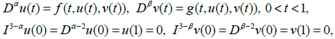
where 2 <α ,β ≤ 3 and f , g : I × R× R→ R are continuous and D, I denote Riemann-Liouville’s fractional derivative and fractional integral respectively. We use Perov fixed point theorem [9] and Leray-Schauder fixed point theorem to obtain sufficient conditions for existence and uniqueness results. We also provide an example to illustrated our results.

Preliminaries

We recall some fundamental results and definitions [10,11].

Definition 2.1

The fractional integral of order α ∈R⁺ of a function y : (0,∞)→ R is defined by

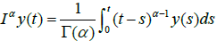
provided the integral converges.

Definition 2.2

The Riemann-Liouville fractional order derivative of a function y : (0,∞)→ R is defined by

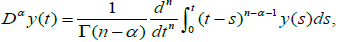
where n = [α ]+1and[α ] represents the integer part of α provided that the right side is point wise defined on (0,∞).

Lemma 2.3

The following result holds for fractional derivative and integral , for arbitrary.

Lemma 2.4

(7) Let X be a Banach space with closed and convex. Let Ω be a relatively open subset of with 0∈Ω and be a continuous and compact(completely continuous) mapping. Then either

1. The mappingT has a fixed point in or

2. There exist μ ∈∂Ωand k ∈(0,1) with Ω = kTu.

Definition 2.5

For a nonempty set Z, a mapping d : Z × Z → Rⁿ is called a generalized metric on Z if the following hold

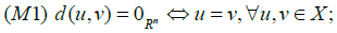
(M2) d(u,v) = d(v,u),∀u,v∈ X, (symmetric property);

(M3) d(x, y) ≤ d(x,v) + d(v,u) + d(u,v),∀x, y,u,v,∈ X, (tetrahedral inequality).

Note: The properties such as convergent sequence, cauchy sequence, open/ closed subset are the same for generalized metric spaces as hold for the usual metric spaces.

Definition 2.6

For an n× n matrix A, the spectral radius is defined by 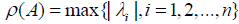, where 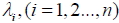are the eigenvalues of the matrix A.

Lemma 2.7

(11), Let (Z, d) be a complete generalized metric space and let T : Z →Z be an operator such that there exist a matrix A∈M with d(Tu,Tv) ≤ Ad(u,v), for all u,v∈Z. If ρ (A) <1, then T has a fixed point Z* ∈Z, further for any Z₀ the iterative sequence Zn +1 = TZn converges to Z₀.

Lemma 2.8

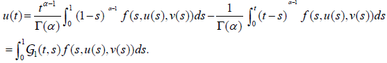
An equivalent Fredholm integral representation of the system of boundary value problems (1.1) is given by (2.1)

, where are Green’s functions given by

(2.2)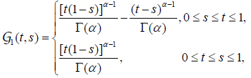

(2.3)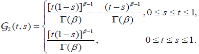

Proof

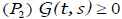
Applying the operator I^α on the first equation of (1.1) and using lemma (2.3), we have

(2.4) .

The boundary conditions and .

Hence, (2.4) takes the form

(2.5)

Similarly, by the same process with the second equation of the system, we obtain the second part of (2.1).

Lemma 2.9

(6) The Green’s function of the system (2.1) has the following properties

is continuous function on the unit square for all

(t, s)∈[0,1]×[0,1];

for all (t, s)∈[0,1] and for all (t, s)∈(0,1);

;

(P₄) there exist a constant γ ∈(0,1) such that

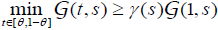for θ ∈(0,1), s∈[0,1] where

.

Existence of positive solutions

Define U = {u(t) | u(t)∈C[0,1]} endowed with the Chebychev norm. Further, define the norms.

Then, the product spaces are Banach spaces. Define the cones by

and

, where J = [θ ,1−θ ], θ ∈(0,1).

Lemma 3.1

Assume that f , g :[0,1]× R× R→ R are continuous. Then (u,v)∈U ×V is a solution of (2.1), if and only if (u,v)∈U ×V is a solution of system of Fredholm integral equations (1.1).

Proof

The proof of lemma (3.1) is similar to proof of lemma (3.1) in [6].

Define T :U ×V →U ×V by

(3.1)

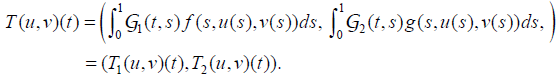
By lemma (3.1) the problem of existence of solutions of the integral equations (2.1) coincide with the problem of existence of fixed points of T.

Lemma 3.2

Assume that f , g :[0,1]×[0,∞)×[0,∞)→[0,∞) are continuous.

Then and , where T is defined by (3.1).

Proof

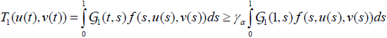
The relation easily follow from the properties (P₁) and (P₂) of lemma (2.9) and all we need to show that holds. For, we have and in view of property (P₄) of lemma (2.9), for all t∈J , we obtain

(3.2)

.

Hence, it follows that

.

Similarly, we obtain

.

It follows that

,

which implies that .

Lemma 3.3

Assume that f , g :[0,1]× R× R→ R are continuous then is completely continuous.

Proof.

We omit the proof, because it is similar to the proof of lemma (3.2) in [6].

Lemma 3.4

Assume that f and g are continuous on [0,1] ×R× R→ R and there exist such that the following holdfor ;

for ;

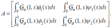
, Where the matrix is defined by

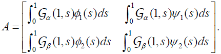
Then the system (2.1) has a unique positive solution .

Proof

Define a generalized metric d :U ×V ×U ×V → R² by

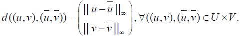
Obviously (U ×V, d) is a generalized complete metric space. For any 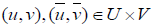using the property (P₃) and (H₃), we obtain

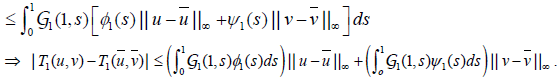
Similarly, we obtain

.

Hence, it follows that

, Where

. Hence by lemma (2.7), the system (2.1) has a unique positive solutions.

Lemma 3.5

Let f and g are continuous on [0,1]× R× R→ R and there exist

satisfying

.

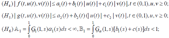
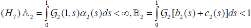Then the system (2.1) has at least one positive solution (u,v) in

.

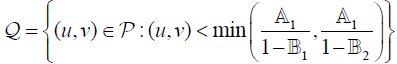Proof

Choose 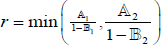and define.

By lemma (3.3), the Operator is completely continuous. Choose and (u,v)∈∂Ωsuch that .

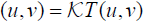Then, by properties (P₁), (P₃) and (H₄), we obtain for all t∈[0,1]

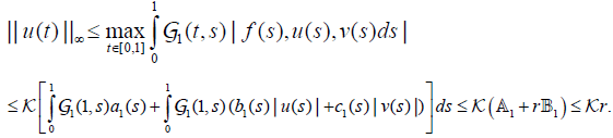
Similarly, we obtain 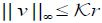, hence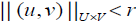, which shows that (u,v)∉∂Ω.Thus by Schauder fixed point theorem,T has a fixed point in .

Examples

Example 4.1

Consider the following coupled systems of boundary value problems

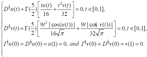Here

.

Moreover

.

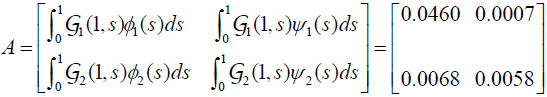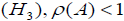
Here, ρ (A) = 4.61×10⁻² <1, hence by lemma (3.4) the BVP(4.1) has a unique solution. For f and g, we have

and by simple calculation, we obtain

. Hence by using lemma (3.5), BVP (4.1) has at least one positive solution.

Conclusion

With the help of Banach theorem and nonlinear Leray Schauder type, we have developed an existence theory to a coupled system of nonlinear FDEs. The concerned results have been successfully obtained and demonstrated by suitable example.

REFERENCES

1. Benchohra M, Graef JR, Hamani S. Existence results for boundary value problems with nonlinear fractional differential equations. Appl Anal. 2008; 87:851-863.
2. Ahmad B, Sivasaundaram S. On four-point non-local boundry value problems of non-linear intigro-differential equations of fractional order. Appl Math Comput. 2010;217:480-487.
3. Rehman M, Khan RA. Existence and uniqueness of solutions for multi-point boundary value problems for fractional differential equations. Appl Math Lett. 2010;23:1038-1044.
4. Zhang S. Positive solutions to singular boundary value problem for nonlinear fractional differential equation. Comput Math Appl. 2010;59:1300-1309.
5. Su X. Boundary value problem for a coupled system of nonlinear fractional differential equations. Appl Math Lett. 2009;22:64-69.
6. Ahmad B, Nieto JJ. Existence results for a coupled system of nonlinear fractional differential equations with three point boundary conditions. Comput Math Appl. 2009;58:1838-1843.
7. Gafiychuk V, Datsko B, Meleshko V, et al. Analysis of the solutions of coupled nonlinear fractional reaction diffusion equations, Chaos Solit Fract. 2009;41:1095-1104.
8. Wang J, Xiang H, Liu Z. Positive solution to nonzero boundary values problem for a coupled system of nonlinear fractional differential equations. Int J Differ Equ. 2010, Article ID 186928.
9. Perov A. On the Cauchy problem for a system of ordinary differential equations, Priblizhen. Metody Resh Dif Uravn. 1964.
10. Miller KS, Ross B. An Introduction to the Fractional Calculus and Fractional Differential Equations. Wiley, New York, 1993.
11. Kilbas AA, Srivastava HM, Trujillo JJ. Theory and Applications of Fractional Differential Equations. Elsevier, Amsterdam, 2006.