Interpolation and Approximation of Functions

Received: 05-Mar-2021 Accepted Date: Mar 16, 2021; Published: 27-Mar-2021, DOI: 10.37532/2752-8081.21.5.24

Citation: Vishnu Narayan M. Interpolation and Approximation of Functions. J Pur Appl Math. 2021; 5(2):5:9.

This open-access article is distributed under the terms of the Creative Commons Attribution Non-Commercial License (CC BY-NC) (http://creativecommons.org/licenses/by-nc/4.0/), which permits reuse, distribution and reproduction of the article, provided that the original work is properly cited and the reuse is restricted to noncommercial purposes. For commercial reuse, contact reprints@pulsus.com

Abstract

Interpolation describes the problem of finding a curve that passes through a given set of real values at real data points, which are sometimes called abscissae or nodes. The theory of interpolation is important as a basis for numerical integration known also as quadrature. Approximation theory on the other hand seeks an approximation such that an error norm is minimized. The Newton interpolation formula has several advantages over the Lagrange formula.

The degree of an interpolating polynomial can be increased by adding more points and more terms. The accuracy of an interpolation polynomial depends on how far the point of interest is from the middle of the interpolation points used.

The Newton form of the interpolating polynomial can be viewed as one of a class of methods for generating successively higher order interpolation polynomials.

The problem with polynomial interpolation is that with increasing degree the polynomial ‘wiggles’ from data point to data point.

Keywords

Mathematics; Approximation; Interpolation; Numerical differentiation

Introduction

Numerical mathematics deals with the approximate or approximate solution of mathematical problems. We distinguish numerical mathematics, numerical linear algebra, numerical solution of nonlinear equations, approximation and interpolation methods, etc. To apply the methods of numerical mathematics, it is necessary to know and analyze the error estimate.

In general, we can say that the problem we solve is called input information and the corresponding result is output information. The process of transforming input into output information is called an algorithm. In this paper, an approximation or approximate match and interpolation or exact matches are treated.

By interpolation we come to functions that pass exactly through all given points, and we use it for a small amount of input data. Interpolation implies the passage of an interpolation function through all given points, while the approximation allows errors to a certain extent, and then we smooth the obtained function.

In the case of interpolation, the problem of determining the function f is called the interpolation problem, and the given points and x_i are called nodes (base points, interpolation points). We choose the function f according to the nature of the model, but so that it is relatively simple to calculate. These are most often polynomials, trigonometric functions, exponential functions and, more recently, rational functions. In practice, it has been shown that it is not wise to use polynomials of degree greater than three for interpolation, because for some functions an increase in the degree of an interpolation polynomial can lead to an increase in errors. Therefore, instead of a high degree of interpolation polynomial, interpolation by parts of the so-called polynomial is used. Spline interpolation.

By approximation, we arrive at functions that pass through a group of data in the best possible way, without the obligation to pass exactly through the given points. The approximation is suitable for large data groups, nicely grouped data, and small and large groups of scattered data.

Approximation occurs in two forms. We know the function f, but its form is complicated to compute. In this case, we select the function information to use. The error of the obtained approximation can be estimated with respect to the true value of the function.

The function f is unknown to us, but only some information about it is known. For example, values at a set of points are known. The substitution function ϕ is determined from the available information, which, in addition to the data itself, includes the expected form of data behavior, ie. Functionϕ. In this case, we cannot make an error estimate without additional information about the unknown function f [1-3].

In practice, we often encounter the variant that the function f is not known to us. It most often occurs when measuring various quantities, because in addition to the measured data, we also try to approximate the data between the measured points.

Some of the mathematical problems can be solved by numerical methods, however, not always with great precision and accuracy. Sometimes the time we have to solve problems is not enough and in that case we use programming methods using a computer. Programming allows you to solve complex tasks with great accuracy and in a short period of time. The ability of a computer to perform a large number of mathematical operations in real time provides great opportunities for numerical mathematics and mathematics in general, and thus the development of science and technology.

All software solutions are integrated systems for numerical and symbolic calculations, graphical presentation and interpretation, and provide support that allows the user to program in an easy way.

Basic Terms

A problem we often encounter in practice is how to calculate the value some function for which we have no analytical expression, but we know its values on some a discrete set of points x₀ < x₁ < x₂ ... < x_i < ... < x_n.

The following questions are asked:

- How in that case to find the value of the function at points those are not from default set?

- How to get this data in the shortest possible time?

We approach the solution of the problem in the following way:

In the data area, i.e. In the interval [x₀, x₁, ..., x_n] unknown function f should to approximate by some simple known function ϕ so it is valid:

ϕ (x_i) f (x_i ), i = 0,1,2,..., n.

Function ϕ it is chosen according to the nature of the model, but so as to be relative easy to calculate. It depends on the parameters a_k, k = 0, ..., n, to be determined by some criterion ϕ (x) =ϕ (x; a₀, a₁,…, a_n).¹

When we function ϕ written in this form, as a function that depends on parameters ak, we can say that we have chosen the general form of the approximation function.

By approximating the set of points, unknown parameters of the function are determined predefined shape (sometimes linear functions, but more often functions of other shapes, such as higher-order polynomials, trigonometric, logarithmic, or exponential function).

The goal of the approximation is to determine the function that “best” describes, ie. at least deviates from the set of default points. Criteria for determining “at least the “deviation” from the set of set points are different least squares. This criterion requires that the sum of the squares of the distances between given points and associated approximations will be minimal.

Unlike approximating a discrete set of given points, on occasion approximation of given functions criterion for “least deviation” criterion is used absolute deviation (which requires the maximum absolute value of the difference between values of the function and its approximation at a given interval) or absolute integral criterion (which requires that the value of the integral of the absolute value of the difference between the function and its approximation be minimal). Such criteria defined are above intervals and are therefore more difficult to assess. Some are often used to calculate them from numerical approximate methods, such as data discretization or numerical integration.

Figure 1. Example of interpolation

Interpolation denotes the method of constructing new data points within the range of a discrete set of known data points (e.g. connected by measurement). Interpolation comes from the word inter between and polos os, axis, or point, knot. Any calculation of a new point between two or more existing point’s data is interpolation.

There are many methods of interpolation, many of which involve adjusting some type of function to the data and then estimating the value of that function at the desired point. One of the simplest forms interpolation is the calculation of the arithmetic mean from the values of two adjacent points how a point in their midpoint would be determined.

Figure 2. Example of approximation

A special case of the approximation problem is the interpolation of functions, where it is required that at certain points, or interpolation nodes, the values of the function f coincide with the values of the approximating function g. In the more general case of interpolation, the values of certain derivatives of the two functions are also required to coincide.

In order to estimate the closeness of the original function f to the approximating function g, metrics of various function spaces are used. Usually, these are the metric for the space C of continuous functions, known as the uniform metric, and the metrics for the spaces Lp of functions with integrable path power, where ρ≥ 1. In these spaces the distance between f and g is determined (for functions defined on the interval [a, b]) according to the formulas.

The problem most frequently encountered and best studied is that of approximating functions by means of polynomials—that is, by expressions of the form.

The approximation theory of functions, also called the constructive theory of functions, is concerned with approximate representation of functions as well as the study of functions on the basis of their approximate representations. Problems in the approximation of elements in banach and general metric spaces are usually also included in the approximation theory of functions.

The approximation theory of functions originated with the work of P. L. Chebyshev. He introduced one of the principal concepts of the theory— the concept of the best approximation of a function by polynomials—and he obtained a number of results concerning best approximations. The best approximation of a continuous function f(x) by the polynomials.

Function Interpolation

Interpolation is generally a term that refers to the process of inserting between two values. In numerical analysis, this expression is used for the procedure by which a new, usually simpler, function is inserted between two known values of a function so that this value does not deviate from the given one by more than some desired limit. The basic problem of interpolation is the existence of a function that has given values f_k at points x_k. We call points (x_k, f_k) interpolation nodes, and function f an interpolation function.

Due to the simplicity of the polynomial function, the term interpolation most often refers to the interpolation of a real function by an algebraic polynomial. The simplest form of an interpolation polynomial is R (x) = a_o + a₁x + ... + a_mx^m. Lagrange’s interpolation polynomial is also known, as well as Newton’s interpolation polynomial.

Lagrangian interpolation

The Lagrangian method of polynomial interpolation uses Lagrangian polynomials to fit a polynomial to a given set of data points.

The following points are given: 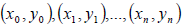, gde su: y_i = f (x_i), i = 0, 1, ... , n. Lagrangian interpolation polynomial of degree ≤ n which goes through these points is:

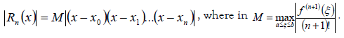
The interpolation error is determined by the formula:

Interpolation by Lagrange polynomials is a procedure in which for n +1 points with the help of Langra’s polynomials it is necessary to find new values of some unknown function or function whose calculation is too difficult (time-consuming or even impossible) [4-8].

The idea behind the procedure is very similar to other methods (Newton’s method, for example): Starting from known points, a new basis of a space is constructed. Then the given function (ie its known values for the given points) is transformed into that new space. A little more informally speaking, it is made into a polynomial, and it serves primarily as a model. This gives a new, approximate function (polynomial) that can be calculated.

Newton’s interpolation

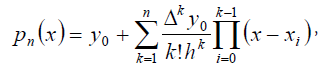
In the mathematical field of numerical analysis, a Newton polynomial, named after its inventor Isaac Newton, is an interpolation polynomial for a given set of data points. The Newton polynomial is sometimes called Newton’s divided differences interpolation polynomial because the coefficients of the polynomial are calculated using Newton’s divided differences method.

In the Newton interpolation, when more data points are to be used, additional basis polynomials and the corresponding coefficients can be calculated, while all existing basis polynomials and their coefficients remain unchanged. Due to the additional terms, the degree of interpolation polynomial is higher and the approximation error may be reduced (e.g., when interpolating higher order polynomials).

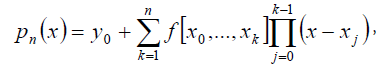
Newton’s interpolation polynomial with divided differences has a shape

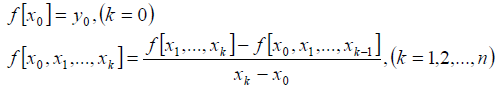
Where the difference of order k is divided, in the notation f[x₀, x₁, ... , x_k], defines as:

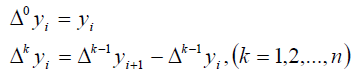
Newton’s interpolation polynomial of the first kind (with decreasing finite differences) is given by:

Where the descending finite differences of order k are defined by:

Newton’s interpolation polynomial of the second kind (with increasing finite differences) is given by:

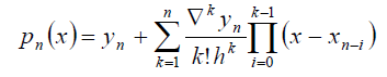
Where the increasing finite differences of order k are defined by:

In comparison, in the Newton interpolation, when more data points are to be used, additional basis polynomials and the corresponding coefficients can be calculated, while all existing basis polynomials and their coefficients remain unchanged. Due to the additional terms, the degree of interpolation polynomial is higher and the approximation error may be reduced (e.g., when interpolating higher order polynomials) [9].

Least squares method

A mathematical procedure for finding the best-fitting curve to a given set of points by minimizing the sum of the squares of the offsets (“the residuals”) of the points from the curve. The sum of the squares of the offsets is used instead of the offset absolute values because this allows the residuals to be treated as a continuous differentiable quantity. However, because squares of the offsets are used, outlying points can have a disproportionate effect on the fit, a property which may or may not be desirable depending on the problem at hand.

Function y = f (x) we approximate by a linear combination of functions

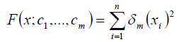
The error function at an arbitrary point x is then . Constant, which need to be found, we determine from the condition to obtain the minimum function of the sum of the squares of the errors (on which the least squares method is based). That is, we are looking for a minimum function:

This function has a minimum if the partial derivatives are per equal to zero. That is:

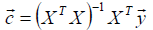
All this written using matrices has the following form:

, where are they:

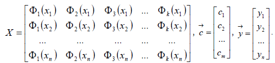
Required constants we determine according to the formula

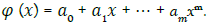
In polynomial function approximation have a shape x^k-1, wherein k = 1,...,m.

The least squares method is one of the most important methods for processing experimentally obtained results. Regression equations, regression analysis, try to draw the optimal curve in the scatter diagram of the results, i.e. the direction of regression that will best describe the relationship of the observed variables. In Figure 1 we see one such diagram before drawing the regression direction.

Figure 3. Scattering diagram

If we show all the data obtained experimentally in the diagram, we would get an arrangement of points through which it is possible to draw an infinite number of directions. Each of the directions would be determined by the corresponding equation with its own parameter values.

In the mathematical field of numerical analysis, interpolation is a type of estimation, a method of constructing new data points within the range of a discrete set of known data points.

In engineering and science, one often has a number of data points, obtained by sampling or experimentation, which represent the values of a function for a limited number of values of the independent variable. It is often required to interpolate, i.e., estimate the value of that function for an intermediate value of the independent variable.

A closely related problem is the approximation of a complicated function by a simple function. Suppose the formula for some given function is known, but too complicated to evaluate efficiently. A few data points from the original function can be interpolated to produce a simpler function which is still fairly close to the original. The resulting gain in simplicity may outweigh the loss from interpolation error.

Interpolation in the mathematical field of numerical analysis means a method of constructing new data points within the range of a discrete set of known data points. In engineering and science, interpolation often has many data points collected by experimentation, so it tries to create a function that roughly corresponds to those data points. This is called curve adjustment or regression analysis. Interpolation is a specific case of curve fitting in which a function must pass accurately through data points [10].

Another problem that is closely related to interpolation is the approximation of a complex function by a simple function. Assuming we know a function that is too complex to estimate efficiently, then we could select a few known data points from the complex function, then create an overview table and try to interpolate those data points to construct a simpler function.

Of course, when we use a simple function to calculate new data points, we usually do not get the same result as when we use the original function, but depending on the problem domain and the interpolation method used to obtain simplicity, an error occurs.

It should be noted that there is another completely different type of interpolation in mathematics called “operator interpolation”. The classic results around operator interpolation are the Riesz-Thorin theorem and the Marcinkiewicz theorem. There are also many subsequent results.

Interpolation comes from the word inter, which means between and polos os, which means axis, point, node. Any calculation of a new point between two or more existing data points is an interpolation.

There are many methods of interpolation, many of which involve adjusting some type of function to the data and then estimating the value of that function at the desired point. This does not preclude other methods such as statistical methods of calculating interpolated data[10].

One of the simplest forms of interpolation is to calculate the arithmetic mean from the values of two adjacent points in order to determine the point in their mean. The same result is obtained by determining the value of the linear function at the midpoint.

Approximation of Functions

Approximation of functions is a mathematical term that represents the case when a given function f needs to be replaced by another function g on some set. A somewhat less formal description of the approximation of a function is that it is a function that is not exactly the same as the initial one, but is much easier to calculate, and is sufficiently accurate in the desired interval. This sufficiently accurate, yet easily calculable function is usually a polynomial [11].

The problem of approximating the function f by the function g is reduced to determining the values of the parameters a₀, a₁, ... a_n. The function approximation can be linear or nonlinear in parameters. Depending on the criteria for the selection of approximation parameters, we distinguish several types of approximation, but the main ones are: Interpolation, RMS approximation.

Approximation of functions

The problem of approximating the function comes down to determining the values of the parameters from a₀, a₁,… a_n. The approximate function can be linear or nonlinear.

Linear approximation functions

The most commonly used forms of linear approximation functions are:

1. Algebraic polynomials, , k = 0,..., m, that is

2. Trigonometric polynomials, which are suitable for approximation of periodic functions. For the function is taken as the (m + 1) function on the set ,

Where k = 0,..., m.

3. In parts, polynomials, the so-called spline functions that are reduced to low-degree polynomial. These polynomials are at all subintervals of the same degree, that is where x₀,...,x_n default points.

Nonlinear approximation functions

We write nonlinear approximation functions in the form

They have a nonlinear dependence on the parameters of the approximation function a₀,...,a_m. Determination parameters a_k usually leads to systems of nonlinear equations or nonlinear problems optimization.

The most commonly used forms of nonlinear approximation functions are:

1. Exponential functions 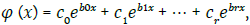which they have n = 2r + 2 independent parameters. These functions have application in various branches as well which are biology, economics, medicine, and can describe the processes of growth and extinction in population.

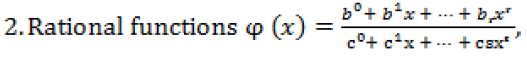
Which have better approximation properties than polynomials. In this form of approximation, the number of independent parameters is n = r + s + 1.

When we create a confidence interval, it’s important to be able to interpret the meaning of the confidence level we used and the interval that was obtained. The confidence level refers to the long-term success rate of the method, that is, how often this type of interval will capture the parameter of interest.

If a confidence interval is given, several conclusions can be made. Firstly, values below the lower limit or above the upper limit are not excluded, but are improbable. With the confidence limit of 95%, each of these probabilities is only 2.5%. Whatever the size of the confidence interval, the point estimate based on the sample is the best approximation to the true value for the population. Values in the vicinity of the point estimate are mostly plausible values. This is particularly the case if it can be assumed that the values are normally distributed.

The goal of the approximation is to determine the function that “best” describes, i.e. deviates the least from the set of set points. The criteria for determining the “smallest deviation” from a set of set points are different. For example, the least squares criterion is used. This criterion requires that the sum of the squares of the distances between the given points and the corresponding approximations be kept to a minimum.

Unlike approximating a discrete set of given points, when approximating given functions the criterion for “smallest deviation” uses the criterion of absolute deviation (which requires the maximum absolute value of the difference between the value of the function and its approximation at a given interval) or absolute integral criterion (which requires that the value of the integral of the absolute value of the difference between the function and its approximation be minimal). Such criteria are defined over intervals and are therefore more difficult to assess. Some of the numerical approximate methods, such as data discretization or numerical integration, are often used to calculate them.

Conclusion

In technique, the approximation occurs in two essentially different forms. The first form is when we know the function but its form is too complicated to compute. In that case, we select some information about the function and determine the approximation function according to some criteria. When we talk about this form of approximation we can choose the information about the function we will use. The second form is when we do not know a function but only some information about it, for example, values on some discrete set of points. The replacement function is determined from the available information. In addition to the data itself, this information includes the expected form of function behavior. We use the first form in theory for the development of numerical methods based on approximation. The second form is more common in practice. For example, when measuring some quantities, in addition to the measured data, we try to approximate the data that are “between” the measured points. A problem that can occur when interpolating with these methods is if the function has sudden changes. In that case, it is necessary to reduce the area of consideration or use e.g. interpolation splines exactly between or around the points that oscillate the most. Regardless, we cannot derive a single general procedure that would be applicable to all cases. Each case needs to be analyzed for itself, the scattering points analyzed, and the most favorable method chosen to give the most accurate results.

Finally, we can say that interpolation is useful in cases where it is known to us only a certain number of values of one function, and we need the values of that function in others points, as well as in the case where the original function is too complex to calculate.

REFERENCES

1. Ivansic I. Numericka matematika, Element, Zagreb. 1998.
2. Vukovic D. Numericka analiza-interpolacija i ekstrapolacija. 2017.
3. Lesić M. Aproksimacija i interpolacija funkcija. 2017.
4. Bojović DR, Sredojević BV, Jovanović BS. Numerical approximation of a two-dimensional parabolic time-dependent problem containing a delta function. JCAM. 2014; 259:129-37.
5. Žitnik T. Neville-ov postupak interpolacije. 2001.
6. Timan AF. Teoriia priblizheniia funktsii deistvitel'nogo peremennogo. Fizmatgiz. 1960.
7. Bergh J. An introduction. Interpolation Spaces. 1976.
8. Jeffreys H, Jeffreys BS. Lagrange’s interpolation formula. Methods of mathematical physics. 1988; 3:260.
9. Press WH, Teukolsky SA, Vetterling WT, et al. Numerical recipes in C++. The art of scientific computing. 1992;2:1002
10. Davis PJ. Interpolation and approximation. Courier Corporation; 1975.
11. Taibleson MH, Nikol′ skiĭ SM. Approximation of functions of several variables and imbedding theorems. Bulletin of the American Mathematical Society. 1977; 83:335-343.