
Measuring Nigeria’s output gap: An application of Kalman filter
Received: 05-Apr-2022, Manuscript No. puljpam-22-4708; Editor assigned: 08-Apr-2022, Pre QC No. puljpam-22-4708(PQ); Accepted Date: May 03, 2022; Reviewed: 22-Apr-2022 QC No. puljpam-22-4708(Q); Revised: 29-Apr-2022, Manuscript No. puljpam-22-4708(R); Published: 06-May-2022, DOI: 10.37532/2752-8081.22.6.3.9-15
Citation: Uzoagulu PC, Onuigbo NF. Measuring Nigeria’s output gap: An application of Kalman filter. J Pure Appl Math 2022;6(3):9-15.
This open-access article is distributed under the terms of the Creative Commons Attribution Non-Commercial License (CC BY-NC) (http://creativecommons.org/licenses/by-nc/4.0/), which permits reuse, distribution and reproduction of the article, provided that the original work is properly cited and the reuse is restricted to noncommercial purposes. For commercial reuse, contact reprints@pulsus.com
Abstract
The deviation between an economy’s estimated potential output and its actual level of output is known as the output gap. The goal of assessing the output gap is to determine the scope or limit for long-term non-inflationary growth and to assess policymakers’ opinions on macroeconomic policies. Using the state-space model and Kalman filtering, the study used seasonally adjusted quarterly and annual GDP data from Nigeria. In order to state the predictability of output, the paper extended the univariate model to a multivariate model. However, we used the univariate Hodrick-Prescott (HP) filter as a baseline for comparing the output gap. The result shows that the gap size varies depending on the approach applied. As a result, the model shows that inflation outperforms unemployment as the quantitative measure of Nigeria’s output gap. The results were satisfactory, and the univariate unobserved component utilizing the Kalman filter, surprisingly, yielded significant outcomes toward the output gap. The output gap estimation also reveals sensitivity due to the inclusion of unemployment in the quarterly data. This implies that policymakers should avoid depending on one approach of estimating output gap.
Key Words
Output gap, Kalman filter, State-space, Inflation, Unemployment
Introduction
When a country is in a crisis or undergoing a downturn, the production of goods and services decreases, whereas when the economy is booming, output increases. Economists and policymakers are generally concerned not just with the ups and downs of the GDP business cycle, but also with whether it is above or below its potential [1]. The output gap is a metric that evaluates both economic oscillations and economic efficiency. The output gap, by definition, is the deviation between an economy’s expected productive potential (also known as “potential output”) and its actual output levels. In literature, a variety of potential output definitions have been proposed, including definitions that include the level of production at full employment, or a maximum output without inflationary pressure, or the maximum number of products an economy can develop or generate when operating at full capacity, and the maximum output using all factors of production [1-3]. Similarly, to how GDP can rise and fall, the output gap can also rise and fall (positive and negative). Neither is, however, ideal. That the output gap is positive, means when output surpasses its potential, capacity constraints are exceeded, and inflation rises. A negative output gap, on the other hand, is seen as spare capacity for the economy, putting downward pressure on inflation over time, [4]. As a result, it is expected that if the gap remains unchanged, inflation will likely remain stable. This relationship tends to attract central banks to monitor the variables with the aim of regulating their size in order to forecast future prices and take precautionary policy measures.
The following is a summary of the rest of the paper: Section 2 briefly examines literature as well as background information on Nigeria’s output gap, inflation, and unemployment rate. Section 3 details the data and methodology employed, then section 4 reveals the empirical result and section 5 concludes.
Literature Review
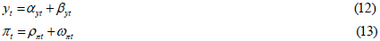
Brief Background on output gap, inflation and unemployment
Despite the economy’s rise in the mid-70s and early-80s as a result of the discovery and exploitation of oil, the country experienced significant and fluctuating inflation. Since the 70s, the high growth of inflation has been attributed to largely the increase of money supply and some factors (such as, wage increase, changes in terms of trade, climate changes, production structure and currency devaluation) considering the structural characteristics of the nation’ economy [5]. However, the oil boom was short-lived, especially after the economy’s primary sectors were abandoned, [6]. In the mid-80s, the economy was struck sharply by a drop in oil revenue, putting the government in a difficult position when it came to budget financing. The government due to this problem, responded by launching the Structural Adjustment Programme (SAP) in 1986. Inflation quickly rose to 50% in the late 1980s, but then fell to about 7.5% in 1990. In 1995, it also reached a record high of 72.8%, causing some analysts to criticize Central Bank of Nigeria’s monetary policies and inability to manage inflation. The high inflation rise is attributed to a limited foreign exchange, a surplus money supply, excess scarcity in commodity supply, a high level of corruption, and, lastly, ongoing labour and political instability as a result of the June 1993 elections being canceled [7-8]. However, from 2013 to 2015, the inflation rate remained steady in the single digits, while real output increased by an average of 6%.
Over time, the profile of Nigeria’s unemployment rate has matched that of inflation. Nigeria’s unemployment rate, on the other hand, has been steady in the single digits since 1980, with the exception of 1984, when it was 10%. However, it peaked at 22.6% in 2018, and increased further to 33.3% as at the last quarter of 2020. The rising number of school graduates without job opportunities, an employment freezes in many public and private sector businesses, and the Nigerian government’s poor capital budget allocation are all contributing factors to the rising unemployment rate [9]. In contrast to the preceding explanation, Nigeria’s output is placed among the fastest rising in emerging economies of Africa.
Brief Empirics
Using quarterly US data, investigate empirically the validity of the extended New Keynesian Phillips Curve (NPKC) model in explaining output gap inflation dynamics. The output gap plays a statistically important part in creating inflation in the stylized NPKC model, thus, the study reveals evidence of serial correlation [10]. Using a variety of statistical techniques, examines Kenya, Ethiopia, Tanzania, and Uganda’s estimated potential output and output gaps. Techniques employed include the linear method, “Hodrick-Prescott filter”, frequency domain filters, and univariate unobservable component models. The findings show that all of the countries assessed the variables equally [11]. The estimated potential output and its related output gaps are completely consistent with the historical boom-bust cycles of all four nations, indicating a sharp display of business cycle turning points rather than the smooth patterns seen in industrialized economies. Between the first quarter of 1980 and the last quarter of 2008, examine the linear trend model, HP filter, and Structural Vector Auto regression (SVAR) to analyze Nigeria’s potential output [12]. The output gap measure obtained from the Structural Vector Auto regression (SVAR) model appears to be the most accurate forecaster of Nigeria’ inflation when compared to the other two techniques.
Using annual data from 1970 to 2006, calculated the output gap-inflation equation in Arab Gulf Cooperation Council countries (AGCC) [13]. The results show that the total output variable has no explanatory capacity for inflation in these nations and isn’t a strong measure of national inflation, with the exception of Saudi Arabia and Oman. Thus, in these countries, there is indeed a link between the output gap and inflation. To estimate Japan’s growth from quarter one of 1980 to quarter three of 2002, utilizes the HP filter [14]. The author compares the results of Japan’s coincident index and Tankan (shorthand for kigyō tanki keizai kansoku chōsa, known as ‘short term economic survey of enterprises’), in order to ensure that the estimated output of the economic cycle is consistent. As a result, the estimated output potential and the resulting output gap are similar to the coincident index and Tankan.
Employs US quarterly data from the second quarter of 1959 to the first quarter of 2013, to study the impact of the output gap on inflation dynamics that are asymmetric in size and sign [15]. To analyze the effect of fluctuations in the output gap on inflation, the author used error correction technique. According to the findings, only large development in the output gap (increase or decrease) would have a significant impact on inflation. Accordingly, inflation may react to equally to the increase and decrease in the output gap changes because the variances are large. Utilized Hungarian annual data from 1960 to 2002 and quarterly data between 1991 and 2002 to estimate potential output and output gap using a variety of univariate de-trending methods, including the ‘Band-pass filter’, “Hodrick-Prescott filter”, unobserved component models, segmented time-trend, “Beveridge-Nelson decomposition”, and wavelet transformation [16]. The authors focused on the structural breaks that occurred during these intervals and how to remedy the problem. They did, however, introduce a single statistic of potential output by evaluating each strategy that passes both the empirical tool and the expertise judgment, taking into consideration the strength and shortcomings of each method. The findings show that while univariate and economic modelbased approaches differ significantly when it comes to the interpretation of transitional shocks in the period of the 1995 adjustment program, they are both common at other periods.
Use a range of theoretical and empirical methodologies to analyze the potential output and output gaps of the Romanian economy between 1998 and 2008 [17]. The author’s method combines the structural method of the production function with empirical de-trending techniques such as “Hodrick-Prescott”, Kalman filter, and wavelet transformation. As a result, production function factors affect the estimated output growth. Furthermore, with a weight based on the revision stability, the statistical de-trending approaches were combined into a consensus estimate. According to the findings, the growth rate of potential output climbed continuously from 1998 to quarter three of 2008, before declining in the last quarter of 2008. The findings also suggest that from 1998 to the third quarter of 2007, technical progress was the primary driver of potential growth, whereas physical capital was the main driving force in the final period. Despite the central bank’s use of the output gap and potential output (which is unobserved), Nigeria still lacks significant research contributions. As a result, this study contributes to the literature in the following areas, particularly in relation to Nigeria: By integrating inflation and unemployment data with the “State space model and Kalman filter”, to measure the output gap. This new technique will be used to overcome some of the flaws in the few previous studies on Nigeria’s output gaps. The “Kalman filter” also aims to address one of the popular approach’s major flaws: the high end-point problem, which stems from the method’s symmetric trending goal over the full sample as well as the numerous limitations that apply both inside and outside the sample.
Data and Methodology
Data
This study made use of both quarterly and annual data. We used the (seasonally adjusted) natural logarithm of Nigeria’s real Gross Domestic Product (GDP), inflation rate, and unemployment rate data over the period, 1980: Q1 to 2020: Q4 for the quarterly data (with a balanced set of a total of 164 quarterly observations). For the annual data, we also used the Gross Domestic Product growth rate, inflation rate and unemployment rate from 1980 to 2020 (with a balanced set of a sum of 41 yearly observations). We estimate the model comparing the “Hodrick-Prescott” filter (1997), statespace representation and “Kalman” filter (1960, 1963) methods using Eviews default settings. The data was obtained from World Bank’s (2020) World Development Indicators [18-20].
Model
The output gap (y) by definition is the deviation between the log of real GDP
(Y), from its potential level 

Methods of Estimation
There are four groups of methods used in estimating output gaps. This includes, the direct output gap measurements using survey data, nonstructural univariate approaches, theory-based or structural methods, and multivariate methods. For this study, we will estimate the output gap with non-structural univariate approaches and multivariate methods.
Non-Structural Univariate methods
They include Univariate “Hodrick-Prescott (HP)” filter and Univariate Unobserved Component.
Univariate Hodrick-Prescott (HP) filter: The Hodrick-Prescott (HP) filter is the most popular and simple filtering approach, owing to its versatility in following the characteristics of trend output fluctuations, but it is also the most generally criticized filter. It calculates time series’ cyclical and trend components. For the full sample of observations (J), the HP filter generates the derived trend component (ϕt) by lowering the combination of the gap between the actual output (βt) , the trend output, and the rate of change in trend output [21].

In equation 2, the first expression sums the squared variances of trend and actual output, while the second expression keeps the trend output growth rate from deviating. The “smoothing parameter” (λ) determines how much weight the deviations are given. As a result, the lower the value, the lower the cost for trend output fluctuations, and the closer the trend output series fits the real output series [22]. As a result, higher values give greater weight to smoothing rates of change in the trend, resulting in less (bigger) volatility in potential growth (output gap) estimates [23]. The smoothing parameter (λ) is commonly set to “1600 for quarterly data and 100 for annual data” when using business cycle data. The aforementioned numbers were selected as a result of “Hodrick- Prescott’s” (HP) prior view on the size of cyclical volatility and the growth trend in US macroeconomic aggregates.
Univariate Unobserved Component model:
State space model: A system of two equations represents the linear-state space model of the dynamics of the n x1 vector αt .
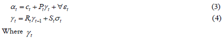
(k x1) is a vector of possibly unobservable variables, where Pt, Rt , and St are comfortable vector and matrices and where εt (weighted by ∀) and σt (weighted by S) are vectors of mean zero Gaussian disturbances. The signal or observation equations are represented in equation (3), while the state or transition equations are represented in equation (4). The two disturbance vectors εt and σt are serially independent and contemporaneously correlated.
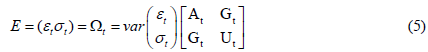
Where At is an k x k proportional variance matrix, Pt is an h × h
proportional variance matrix and Gt is an k × h matrix of covariance. The
specification given from equation (3) to (5) will be generalized by allowing
the systems of matrices and vectors  to rely on
observable explanatory variables Pt and unobservable parameters Ø.
to rely on
observable explanatory variables Pt and unobservable parameters Ø.
• Kalman Filter: The maximum likelihood technique can be used to evaluate the model’s parameters and unobserved components using a state space model and “Kalman filter” [19]. The Kalman filter is a method for ensuring state estimation in a stochastic linear dynamic system. In a state-space model, it is also an algorithm for obtaining a minimum mean square error forecast. The “Kalman filter” is a recursive algorithm for linearly updating the onestep- ahead forecast of the state mean and variance, given new information (that is, measurement knowledge of the system model and statistical descriptions of its inaccuracies, noise, and errors), [24,25].
We will use the “local-level” or random walk with noise model to estimate the trend and cycle breakdown. It is local in the sense that, due to a shock (θt) , the level can change from one period to the next. This so-called local level consists of a stochastic trend (ϕt) and cyclical component (dt) , both of which are supposed to follow an Autoregressive (AR) (2) process:
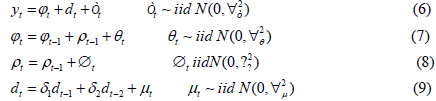
Where , are individual white noise processes, and òt is an
irregular white noise in equation (6) (which might be evaluated for statistical
significance of its variance unless
are individual white noise processes, and òt is an
irregular white noise in equation (6) (which might be evaluated for statistical
significance of its variance unless  is not statistically significant from zero,
in which case the measurement error can be removed). In equation (6), the
non-stationary trend component (ϕt)
is represented as an approximation
to the local linear trend model. Thus, the level form innovation (ϕt) , are
represented by
θt, whereas
is not statistically significant from zero,
in which case the measurement error can be removed). In equation (6), the
non-stationary trend component (ϕt)
is represented as an approximation
to the local linear trend model. Thus, the level form innovation (ϕt) , are
represented by
θt, whereas  is the first difference form or growth rate
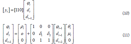
innovation. Equation (6) can be expressed in state space structure, using
both (ϕt) and dt as unobserved state variables as follows:
is the first difference form or growth rate
innovation. Equation (6) can be expressed in state space structure, using
both (ϕt) and dt as unobserved state variables as follows:
Multivariate Unobserved Components model
Variables other than GDP are usually based on relationships established by economic theory in a multivariate model. In essence, extending a univariate UC model to a multivariate model resolves criticisms that a univariate model of real gross domestic product (RGDP) may understate output predictability [26]. Additional variables are useful if cyclical movements in actual output have a different effect on them than movements in potential output. The “Okun’s law” and the “Phillips curve” are the most commonly used variables to augment the univariate output filter. We will create a correlated unobserved component model for output and inflation for quarterly data, as well as output and unemployment for annual data, based on the above explanation.[26-28] all examined output and unemployment. The cyclical output movement is evaluated using a multivariate unobserved components model, according to Clark (1989), in which output and unemployment or inflation (the variables employed) separately have trend components but share a cyclical component [27].
The trend component is the steady-state level after all transitory movements have been removed, whereas the cycle component includes all transitory movements and is presumed to be stationary:
For each trend component (αyt , ρπt ) a random walk permits for persistent movement in the series.
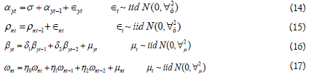
The cyclical inflation component ωπt is presumed to be a function of the present and previous cyclical output components, and all errors are assumed to be white noise. Unemployment’s trend and cyclical component are both characterized in the same way. Equation (17) is based on an equation for the Philips curve, following, and assumes that inflation expectations are based on the previous levels of consumer prices and imported goods and services [29,30]. Kuttner (1994) extended the univariate unobserved components model of output by adding details about the output gap included in the Phillips curve while presuming inflation to be lower than the expected rate when the output gap is negative [29]. The above equations could be expressed in a state-space structure if all variables are assumed to be unobserved as follows:
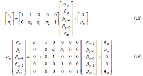
Incorporating inflation data into the model could further enhance the basis for large transitory changes in RGDP, according to Clark [31]. Additionally, integrating inflation data may bring the output gap estimation closer to its definition which is rooted on stable inflation. Thus, the component would connect the cyclically high inflation rates to the output component which is transitory, [23].
Estimation Results
Descriptive Statistics (Annual data)
Source: Author’s estimates
According to table 1, the average annual growth rate, inflation rate, and unemployment rate over the period of study were 3.27%, 18.7 % and 7.08 % respectively. The double-digit inflation rate could be due to the economic crisis, particularly during the pandemic (3rd and 4th quarters of 2020), in addition to the lack of appropriate monetary and fiscal policies by the Central Bank of Nigeria to address the issue. The yearly GDP value has a maximum of 33.7 and a minimum of -13.1. GDP, inflation, and unemployment are not normally distributed, according to the Jarque-Bera (JB) statistics.
TABLE 1 Individual summary statistics
| Statistics | GDP | Inflation | Unemployment |
|---|---|---|---|
| Mean | 3.2755 | 18.753 | 7.0867 |
| Median | 3.4447 | 12.217 | 6.777 |
| Maximum | 33.735 | 72.836 | 22.6 |
| Minimum | -13.128 | 5.3822 | 3.5 |
| Std. Dev. | 7.1857 | 16.726 | 3.2769 |
| Skewness | 1.3614 | 1.8629 | 3.4005 |
| Kurtosis | 9.7454 | 5.3122 | 15.6016 |
| Jarque-Bera | 90.394 | 32.848 | 350.302 |
| Probability | 0 | 0 | 0 |
| Observations | 41 | 41 | 41 |
Univariate Hodrick Prescott (HP) estimates
Many authors have empirically demonstrated that trend-cycle decomposition has an analogous state-space form, including [32]. Demonstrated how the Hodrick Prescott (HP) filter is identical to the smoothed trend component derived from the actual local linear trend specified in equations (6) to (8) above [33]. We used the conventional value of λ=100 for annual data in this analysis, as well as λ=50 and λ=40 to assess the robustness and performance of the result. Table 2 shows that the output gap for λ (40, 50, and 100) were statistically negative at 1% and 5% significance level. While the output gap for the three values are negative, their potential gap values are positive. In essence, for a developing country like Nigeria, smoothing parameter values greater than λ =100 may not be appropriate where the trend might not be smooth.
The graph shows that both the low and high values of λ have a plausible volatility. The higher the value of λ, as previously indicated in section (3.3.3.1), the larger the variations in the estimations of output gaps, as shown in figure 1. In other words, the extent (size) of the gap changes as the smoothing parameter changes, and the output changes as the corresponding degree and adjustment of peaks and troughs changes. For example, in 2004, the high smoothing weight produced output that was far above its potential at 25%, whereas in 1997, the low smoothing weight produced output that was substantially below its potential. It also shows that at 1981 and 1897, the three values of λ were below the potential output. According to the measure, output gap is low, ranging around zero from 1993 to 2000 and 2006 to 2020. From 1981 to 2016, it shows 9 years of fluctuations below its potential. Similarly, from 1980 to 2004, there were 7 years of fluctuations above its potential output, with a larger estimated output gap.

Figure 1: Output gap using UHP Filter: Annual data
However, one of the above filter’s main flaws is its high end-point problem, which reflects the method’s symmetric trending goal across the entire sample as well as the various limitations that apply both within the sample and at its borders. When the prime focus is aimed at the final observations in the sample in order to infer conclusions for policy recommendations and future projections, the severity of the problem becomes apparent. In essence, this bias can be eliminated by including an adequate amount of GDP predictions in the fundamental data series [34,35].
Univariate Unobserved Component (Annual data)
While the potential output is positive, the estimated output gap is negative and at 1% statistically significance level, as seen in table 2.
TABLE 2 Maximum likelihood estimates of output and potential gap (Annual data)
| Estimation method | Output gap(dt) | Potential gap(ϕt) |
|---|---|---|
| Hodrick Prescott | ||
| 40 | -4.6462* | 2.8284 |
| 50 | -4.7133** | 3.0495 |
| 100 | -4.1287** | 3.5398 |
| Kalman estimates | ||
| Univariate GDP | -0.6414*** | 3.1466 |
| Multivariate with Inflation | 1.3241*** | -4.6324*** |
| Multivariate with Unemployment | 3.6175*** | 5.0091*** |
The Kalman filter graph is equivalent to the Hodrick-Prescott graph in figure 1 for annual output gap. The graph figure 2 illustrates that there were four major troughs in 1981, 1987, 2016, and 2020. It also shows that there were five peaks where the output gap outperformed its potential. The largest positive gap was around 28% in 2004, while the output gap was below its potential in 1981. Specifically, the output gap estimation has been alternating near zero following year 2005, with a severe slowdown of roughly 10% in 2020, possibly due to the Covid-19 epidemic.

Figure 2: Univariate unobserved component (Annual data)
Multivariate Unobserved Component
Both the calculated multivariate UC output gap and potential output are positive, according to Table 2. Although the estimated potential gap is significant at 1%, the output gap is statistically insignificant.
When information regarding unemployment and inflation are used Figures 3 and 4, the profile of the output gap is inconsistent with the univariate UC, and the amount of the gap varies at times. When unemployment data is included, for example, the estimated output gap shows three large slowdowns in 1981, 1984, and 2020. The graph also illustrates that the estimated output gap was practically zero from 1999 to 2013. It also shows three peaks of roughly 10%, 3%, and 2% respectively in 1983, 1986, and 2018.

Figure 3: Multivariate Unobserved Component (Unemployment)

Figure 4: Multivariate Unobserved Component (Inflation)
Furthermore, when inflation data is included, demand appears to be weaker from 1999 to 2020, presumably due to upward pressure on the Headline index, which is mostly due to rising divisions that contribute to the Core Sub-index in Nigeria. According to the National Bureau of Statistics (NBS), prices in most major non-food sectors (such as energy, housing, clothing and footwear, and so on) have increased at a quicker rate. Another assumption could be the sharp drop in crude oil production, which has been coupled by capital reversals as a result of investors loss of confidence. Because of the country’s recession, which was mostly caused by severe external shocks worsened by its poorly-diversified economic base, the output gap was below its potential in 2016 and 2017 [36]. In addition, the two distinct business cycle state peaks occurred in 1983 and 1986, with a surplus of 12% and 3%, respectively.
Descriptive Statistics (Quarterly data)
Similar to the annual summary statistics above, the average value of GDP, inflation rate, and unemployment rate over the period under study are 3.27%, 18.7%, and 7.08%, respectively, according to table 3. Annual GDP value has a maximum of 33.7 and a minimum of 13.1. Unemployment has a standard deviation of 33.2, whereas inflation has a standard deviation of 16.8. GDP, inflation, and unemployment are not normally distributed, according to the Jarque-Bera (JB) statistics.
Table 3 Individual Summary Statistics
| Statistics | GDP | Inflation | Unemployment |
|---|---|---|---|
| Mean | 3.2755 | 18.753 | 7.0867 |
| Median | 3.1224 | 12.639 | 6.7572 |
| Maximum | 35.844 | 76.426 | 23.759 |
| Minimum | -14.375 | 0.667 | 2.8929 |
| Std. Dev. | 7.385 | 16.869 | 3.3247 |
| Skewness | 1.2569 | 1.8321 | 3.3578 |
| Kurtosis | 8.89 | 5.3069 | 15.567 |
| Jarque-Bera | 280.25 | 128.12 | 3187.4 |
| Probability | 0 | 0 | 0 |
| Observations | 164 | 164 | 164 |
Univariate Hodrick Prescott (HP) Estimates
We used the value of λ=40 for quarterly data in this analysis, as well as the values of λ=50 and λ=80. It has been figure 5 observed that a greater value will produce a spurious result (result not reported). Table 4 shows that the potential output for λ=40 was negative, whereas the potential outputs for λ=50 and λ=80 were positive. At the 5% and 10% levels, the estimated output gap of the three values was negative and statistically significant. In essence, for a developing country like Nigeria, smoothing parameter values less than λ=100 may be favourable. Despite this, as previously stated, the use of HP filters has several drawbacks.

Figure 5: Output Gap using UHP Filter: Quarterly data
Table 4 Maximum Likelihood Estimates of Output and Potential Gap (Quarterly data)
| Estimation method | Output gap (dt) | Potential gap (ϕt) |
|---|---|---|
| Hodrick Prescott | ||
| 40 | -3.6356* | -0.0001 |
| 50 | -3.4104** | 0.1704 |
| 80 | -3.0216** | 0.5522 |
| Kalman estimates | ||
| Univariate GDP | -9.5717*** | 5.9343** |
| Multivariate with Inflation | 0.5288** | -5.4764*** |
| Multivariate with Unemployment | 0.2345 | -5.5894*** |
The graph reveals an interesting fact. According to the HP graph, the lower smoothing weight of λ=40 results in a bigger fluctuation and a surplus of more than 22%, λ=50 indicates a surplus of 20%, and the higher smoothing value indicates a surplus of less than 20%. With about 6%, 8%, and more than 17%, the three smoothing weights show three distinct peaks in 1981, 1990, and 2005, respectively. Similarly, in mid-1981, 1987, and 2020, the estimated output gap was greater than its potential.
Univariate Unobserved Component (Quarterly data)
The estimated output gap is negative and at 1% statistically significance level, whereas the potential output is positive and at 5% statistically significance level, according to the UUC results.
The graph figure 6 of the UUC smoothed cycle differs from the graph of the HP filter output gap. The Nigerian economy saw three distinct peaks between 1985 and 1990, with a maximum positive gap of about 30% in 2004, while the output gap was below its potential from 1996 to 2003. The graph also shows a 16-year oscillation around zero from 1982 to 2003, as well as a 7-year oscillation around zero from 2012 to 2020, where the estimated output gap is relatively low.

Figure 6: Univariate Unobserved Component (Quarterly data)
Multivariate Unobserved Component
Table 4 shows that at a 5% level, the estimated multivariate UC with inflation data, output gap is positive and at 1% statistically significance level, the estimated potential gap is negative and statistically significant. When unemployment data is included, however, the potential gap is likewise negative at 1%, although the estimated output gap is positively not significant.
When information about unemployment data and inflation data are used, the profile of the output gap in figure 7 and figure 8 is homogeneous with the multivariate UC, and the size of the gap varies at times. From 1980 to 2020, the graph shows a lot of variations. The graph also illustrates that the output gap was below its potential until after 2016, even before and after the global financial crises. However, between the beginning of the 1990s until 2016, the estimated output gap was negative, with the greatest year being 2019, with a maximum negative output gap of 1.0%. This evidence is consistent with the NBS 2020 abridged labour force survey, which shows that with an increasing labour force population, unemployment increased by 4.1% between the second-quarter of 2018 and the second-quarter of 2020, while underemployment rate increased from 20.1% in 2018: Q3 to 28.6% in 2020: Q2. Other factors comprise the growth of population, specifically among the labour force (from 15-64 years), and the limited number of new employment created. The recent coronavirus outbreak contributed to rising unemployment by disrupting global supply chains; the oil price collapse, which depleted the foreign reserves, led to an increase in exchange rates in Nigeria that relies on imports for non-durable goods and raw materials, finding it challenging for businesses to reach their obligations and, subsequently, dismiss workers. Another factor is a lack of effective school curriculum; particularly the constantly changing environs regarding industrialization, technological advancements, corporate technical abilities, and so on, which has resulted in a skills gap, or a discrepancy in terms of qualifications and skill sets between the supply side of labour and the demand side of labour, [37].

Figure 7: Multivariate Unobserved Component (Unemployment)

Figure 8: Multivariate Unobserved Component (Inflation)
Quarterly inflation and GDP graphs reveal significant volatility and a significant slowdown in the economy. From 1998 through 2020, the estimated output gap is below its potential, with a high output gap of 3.8% in 1995.
Output gap comparison from the three state-space models employed Annual Data
The graph figure 9 depicts the three output gap estimates. HP filter, Univariate unobserved component, and Multivariate unobserved component (unemployment and inflation). The three estimates exhibit some overlap on the estimated output gap, especially at the end-point of the sample. The multivariate unobserved component has the smallest gap, indicating that the corresponding output gap estimates are close to each other and sensitive to the input of unemployment data and inflation data. Simply put, the Kalman filter method generates a more robust multivariate unobserved component than the HP filter. The univariate unobserved component has a large positive output gap of 29 % in 2004 and also has the highest negative output gap of 12% in 1987. Finally, the multivariate unobserved component of GDP and unemployment appears to be moving round zero [38-39].

Figure 9: Output gap comparison
Quarterly Data
The estimated output gap’s profile figure 10 yielded a surprising result. First, both the HP filter and the univariate unobserved component suggest a sizable positive output gap in the fourth quarter of 2015. The multivariate unobserved component with unemployment, on the other hand, yielded zero. This suggests that including unemployment in the model understates GDP predictability, i.e., the corresponding output gap estimates (specifically the multivariate unobserved component) are far apart and reasonably sensitive to the inclusion of unemployment or inflation. However, it appears that at the end-point of the sample, there is agreement across the three estimated output gaps, which all lead to a negative output gap. Finally, the univariate unobserved component implies that in 2004, there was one distinct positive output gap of roughly 32%.

Figure 10: Output gap comparison
Conclusion And Policy Recommendations
The deviation between an economy’s estimated potential output and its particular level of output is called the output gap. The goal of evaluating this gap is to determine the scope or limit for long-term non-inflationary growth and to assess policymakers’ opinions on macroeconomic policies. Using the state-space model and Kalman filtering, the study used seasonally adjusted quarterly and annual GDP data from Nigeria. In order to state the predictability of output, the paper extended the univariate model to a multivariate model. As a result, the model shows that inflation outperforms unemployment as the quantitative measure of Nigeria’s output gap. The results were satisfactory, and the univariate unobserved component utilizing the Kalman filter, surprisingly, yielded significant outcomes toward the output gap. The output gap estimation also reveals sensitivity due to the inclusion of unemployment in the quarterly data. This implies that policymakers should avoid depending on one approach of estimating output gap. Therefore, we recommend that Kalman filter method be included in conjunction with the Central Bank’s current methods for estimating output gaps. It is also recommended that the Central Bank should aim to maximize growth by lowering the inflation rate from approximately 16% to a singledigit figure, taking into account the economy’s peculiarities and structure.
References
- Jahan S, Mahmud AS. What is output gap? Journal of Finance and Development. 2013.
- Okun AM. Potential GNP: its measurement and significance. Cowles Comm/Found 190.1962.
- De Masi MP. IMF estimates of potential output: theory and practice. Int Monet Fund.1997;97(177):1. Google Scholar Crossref
- Yaaba BN. Nigeria’s potential growth and output gap: Application of different econometrics filters. IISTE, J Econ Sustain Dev. 2013;4(13):132-143. Google Scholar
- Masha I. New perspectives on inflation in Nigeria. Econ Financ Rev. 2007;38(2):3. Google Scholar
- Shodipe OT. A comparative analysis on output gap-inflation relation: A new Keynesian approach. 2019. Google Scholar
- Mordi C, Essien E, Adenuga A, et al. The dynamics of inflation in Nigeria. CBN Occas Pap. 2007;32. Google Scholar
- Bawa S, Abdullahi IS. Threshold effect of inflation on economic growth in Nigeria. CBN J Appl Stat. 2012;3(1):43-63. Google Scholar
- Ojima D. Unemployment and economic development in Nigeria. Adv Soc Sci Res J. 2019;6(1):110-21.Crossref
- Zhang C, Osborn DR, Kim DH. Observed inflation forecasts and the New Keynesian Phillips curve. Oxf Bull Econ Stat. 2009;71(3):375-98. Google Scholar Crossref
- Osman M. Estimating potential output gap for East African countries: An eclectic approach. Eur J Econ Finance Adm Sci. 2008;12. Google Scholar
- Patricia A, Milton I, Eugene K. Estimating potential output for Nigeria: A structural VAR approach. Retrieved from. 2009;26. Google Scholar
- Osman M, Louis R, Balli F. Which output gap measure matters for the Arab Gulf Cooperation Council Countries (AGCC): The overall GDP output gap or the non-oil sector output gap? 2008. Google Scholar
- Somchai, A. Japan’s growth: An HP filter approach. Research paper for Econ. Econ Dev Jpn. 2002;614. Google Scholar
- Valadkhani A. Asymmetric size-dependent effects of the output gap on inflation: US evidence from the last half a century. Appl Econ. 2015;47(33):3525-39. Google Scholar Crossref
- Darvas Z, Vadas G. Univariate potential output estimations for Hungary. Magy Nemz Bank Work Pap. 2003;8. Google Scholar
- Moisa A, Ciprian N, Gabriel B. Estimating potential GDP for the Romanian economy. An eclectic approach. Romanian Journal of Economic Forecasting. 2009;13(3),5-25. Google Scholar
- Hodrick RJ, Prescott EC. Postwar US business cycles: An empirical investigation. J Money Credit Bank. 1997;29(1):1-16. Google Scholar Crossref
- Kalman RS. A new approach to linear filtering and prediction problems. J Basic Eng., Transactions ASME. 1960;82:35-45 Google Scholar Crossref
- Kalman, R. S. New methods in Wiener filtering method, in Bogdanoff, J L & Kozin, F (eds), Proceedings of the first symposium on engineering applications of random function theory and probability. New York Wiley. 1963:270-388.
- Araujo CH, Areosa MB, Guillén OT. Estimating potential output and the output gap of Brazil. Anais do xxxii Encontro Nacional de Economia. 2004.
- Claus I, Conway P, Scott A. The output gap: measurement, comparisons and assessment. Reserve Bank N Z. 2000;44:51-54.Google Scholar
- Cerra V, Sweta CS. Alternative methods of estimating potential output and the output gap: An application of Sweden. Int Monet Fund Work Pap. 2000. Google Scholar Crossref
- Ole R. Estimating the output gap for Kenya: A practical guide to some state-space and Kalman filter trend-cycle decompositions. Cent cent bank stud Econ Model Forecast. 2015. Google Scholar
- Fronckova K, Prazak P, Soukal I. Review of Kalman Filter Employment in the NAIRU Estimation. Systems. 2019;7(3):33.
- Sinclair, T. M. Permanent and transitory movements in output and unemployment: Okun’s law persists. Job Market paper. 2004.
- Clark PK. Trend reversion in real output and unemployment. J Econom. 1989;40(1):15-32. Google Scholar Crossref
- Blanchard OJ, QuahD. The dynamic effects of aggregate demand and supply disturbances. Am Econ Rev. 1989;79(4): 655-73. Google Scholar Crossref
- Kuttner KN. Estimating potential output as a latent variable. Journal of business & economic statistics. 1994;12(3):361-8. Google Scholar Crossref
- Gerlach S, Smets F. Output gaps and inflation. Bank of International Settlements mimeo. 1997.
- Clark PK. The cyclical component of US economic activity. Q J Econom. 1987;40(1):797-814. Google Scholar Crossref
- Harvey AC, Trimbur TM. General model based filters for extracting trends and cycles in economic time series. Rev Econ Stat. 2003:85(2):244-55. Google Scholar Crossref
- Harvey AC, Jaeger A. Detrending, stylized facts and the business cycle. J Econom. 1993;8(3):231-47.
- Mise E, Kim TH, Newbold P. On sub-optimality of the Hodrick-Prescott filter at time series endpoints. J Macroecon. 2005;28(1):53-67. Google Scholar Crossref
- Alichi A. A new methodology for estimating the output gap in the United States. Int Monet Fund Work Pap. 2015. Google Scholar Crossref
- Uwatt U, Adebiyi A, Olusegun S, et al. Inflation threshold in Nigeria revisited. CBN Economic and Financial Review. 2018;56(2):1-23.
- Shalihu AA. Unemployment in Nigeria: Policy review and recommendations. 2021.
- Canova F. Detrending and business cycle facts. J Monet Econ. 1998;41(3):475-512. Google Scholar Crossref
- Canova F. Detrending and business cycle facts: A user’s guide. J Monet Econ. 1998;41(3):533-40. Google Scholar Crossref