Revisiting the problem of recovering functions in ℝⁿ by integration on k Dimensional planes

Received: 19-Jan-2018 Accepted Date: Feb 21, 2018; Published: 22-Feb-2018, DOI: 10.37532/2752-8081.18.2.4

Citation: Salman Y. Revisiting the problem of recovering functions in ℝⁿ by integration on k Dimensional planes. J Pur Appl Math. 2018;2(1):12-19.

This open-access article is distributed under the terms of the Creative Commons Attribution Non-Commercial License (CC BY-NC) (http://creativecommons.org/licenses/by-nc/4.0/), which permits reuse, distribution and reproduction of the article, provided that the original work is properly cited and the reuse is restricted to noncommercial purposes. For commercial reuse, contact reprints@pulsus.com

Abstract

The aim of this paper is to present inversion methods for the classical Radon transform which is defined on a family of k dimensional planes in ℝⁿ where 1≤k≤n–2. For these values of k the dimension of the set , of all k dimensional planes in ℝⁿ, is greater than n and thus in order to obtain a well-posed problem one should choose proper subsets of . We present inversion methods for some prescribed subsets of which are of dimension n.

Keywords

Integer; Euclidean space; Hyperplanes; Subset

For an integer n≥2 denote by ℝⁿ the n dimensional Euclidean space. For p∈ℝⁿ and r≥0 denote by|

S (p , x) ={ x ∈ℝⁿ:|s– p |= r }

the hypersphere in ℝⁿ with the center at p and radius r. Let be the unit sphere in ℝⁿ and for every ψ∈S^n-1 denote by the great n–2 dimensional subsphere of S^n-1 which is orthogonal to ψ:

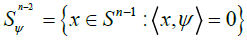
where ❬,❭ denotes the usual inner product in ℝⁿ. For an integer k satisfying 1≤k≤n–1 denote by and by respectively the families of all k dimensional planes (k planes for short) and k dimensional subspaces (i.e., k planes passing through the origin) in ℝⁿ.

For a continuous function f, defined in ℝⁿ, define the k dimensional Radon transform of f by

Where dm_Σ denotes the standard infinitesimal area measure on the k plane Σ.

The main problem and known results

The aim of this paper is to find inversion methods for the k dimensional Radon transform in case where n≥3 and 1≤k≤n–2. That is, we would like to express a function f in question via its k dimensional Radon transform .

In case where k=n–1 the k dimensional Radon transform coincides with the classical Radon transform R which integrates functions on the set of all hyperplanes in ℝⁿ. There is an extensive literature regarding the classical Radon transform where the first results can be tracked down to 1917 when J. Radon showed in [1] that any differentiable function f in ℝ³ can be recovered from its Radon transform (i.e., where our data consists of the integrals of f on hyperplanes in ℝ³). Further results concerning the problem of recovering a function f from in higher dimensions as well as finding uniqueness and range conditions for R have been obtained by many authors and we do not intend to give an exhaustive list of references. Some classical results can be found in [2-4].

For the case where 1≤k≤n–2 and where is defined on the whole family of k planes in ℝⁿ then obviously the reconstruction problem becomes trivial since one can use known inversion methods for the case where integration is taken on hyperplanes in ℝⁿ and the fact that each such hyperplane is a disjoint union of k planes. However, if 1≤k≤n–2 then 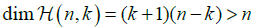and the inversion problem becomes over determined. Thus, in order to obtain a well posed problem one should restrict the domain of to a subset 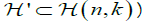for which.

An extensive work and results concerning the problem of determining a function f from in case where the later transform is restricted to various subsets of dimension n have been obtained in [5,6]. In (6, Chap. 4.2) a reconstruction formula was found in case where is restricted to a subset of lines which meet a curve C⊂P(ℝⁿ) (where P(ℝⁿ) is the projective space of all lines in ℝⁿ which pass through the origin) at infinity. The dimension of this subset coincides with the dimension of n in case where n=3.

In (5, Chap. 2.6) and (6, Chap. 4.3) a reconstruction formula was obtained for in case where (3,1) is the set of all lines which intersect a curve which satisfies the completeness condition: each hyperplane which passes through supp(f) intersects Γ transversely at a unique point. In (6, Chap. 4.4) the more general case, where lines are tangent to a given surface in ℝ³, was considered (every curve Γ=Γ(s) can be approximated by the family of surfaces . For cases where integration is taken on planes of dimension k>1 it is shown in (6,Chap. 5.1) how to obtain an inversion formula in case where consists of k planes of the form x+L where L∈C, x∈L^T and C is a k dimensional manifold in .

Main results

In this paper we present three inversion methods for three different prescribed subsets of where for each such subset the problem of recovering a function f, defined in ℝⁿ, from its k dimensional Radon transform is well posed (i.e., the dimension of the manifold H` of k planes is equal to n).

The first inversion method is obtained for a special subset which is determined by fixing k+1 points x₁,…,x_k+1 in ℝⁿ in general position. Each k plane in is determined by taking a point p in ℝⁿ, which is in general position with the other fixed points, and then taking the intersection of the k+1 plane passing through p, x₁,…,x_k+1 and the unique hyperplane which passes through p and its normal is in the direction . We prove that our inversion problem is well posed and provide an inversion method for each function, whose k dimensional Radon transform is defined on this subset , and which satisfies a decaying condition at infinity. The proof of the reconstruction method is purely geometrical and does not use any analytical tools. We find a family of k+1 planes such that the union of these planes is dense in ℝⁿ and such that for every k+1 plane Σ in this family the set of k planes in , which are contained in Σ, is in fact the set of all k planes in Σ. Thus, we can use known inversion formulas for the classical Radon transform, on each such k+1 plane, in order to reconstruct the function f in question.

The second inversion method is obtained for the subset (3,1) of all lines in ℝ³ which are at equal distance from a fixed given point p. We show that our problem is well posed (i.e., in this case ) and obtain an inversion method using expansion into spherical harmonics and exploiting the fact that is invariant under rotations with respect to the point p. Observe that can be also described as the set of lines which are tangent to a given sphere with center at p.

The third inversion method is obtained for the subset (3,1) of all lines in ℝ³ which have equal distances from two given fixed points x and y in ℝ³ (x≠y). Again, we show that our problem is well posed and for the inversion method we exploit the fact that is invariant under rotations with respect to the line l passing through the points x and y. Using this invariance property of we take any hyperplane H, which is orthogonal to l, and expand the restriction f|H, of the function f in question, into Fourier series with respect to the angular variable in H.

We would like again to emphasize that the problem of recovering functions from integration on k planes, which belong to an n dimensional manifold , is not new and the manifolds of lines, corresponding to the second and third inversion problems described above, were already considered in [5,6]. However, the inversion methods presented in this paper are new and can provide new insights on developing other reconstruction methods for more complex subsets of k planes in .

Exact formulations and proofs of the main results

In this section we formulate and prove the inversion methods for the problem of recovering a function f from integration on any subset of k planes from the three subsets which were described in the previous section. For the first subset of k planes we do not give an explicit inversion formula but instead we just assert that every function can be reconstructed from integration on k planes from whereas the inversion method is described in the proof itself. This is because we relyon the reduction to the classical Radon transform from which one can choose many known inversion formulas for this integral transform. The reconstruction methods for the other two subsets are given explicitly.

The description of the subsets of k planes and the inversion methods, for the three subsets described above, are given in the following three subsections. Each subsection is self-contained and the mathematical tools, the main results and their proofs for the reconstruction formulas, for each one of these three subsets, are formulated individually in each subsection.

The case of integration on k planes determined by choosing k+1 points in ℝⁿ

For k+1 arbitrary points x₁,…,x_k+1 in ℝⁿ which are assumed to be in general position, i.e., which satisfy the condition

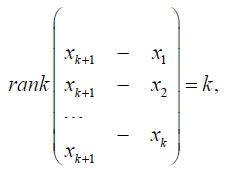[2.1]

denote by H{x₁,…,x_k+1} the unique k plane passing through the points x₁,…,x_k+1. For every x₀∈ℝⁿ\{0} denote by Hx₀ the unique hyperplane whose closest point to the origin is x₀, i.e.,

H_x0={x∈ℝⁿ:⟨x– x₀,x₀⟩=0}.

For every m points x₁,…,x_m in ℝⁿ define the following set

U=U{ x₁,…,x_m}={x∈ℝⁿ:⟨x–x₁,x⟩=…=⟨x–x_m⟩=0}

Observe that in particular 0∈U.

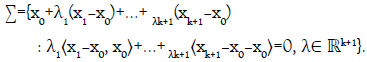
We choose the subset H` in the following way. We fix k+1 points x₁,…,x_k+1 in ℝⁿ which are assumed to be in general position and then, for each x₀∈ℝⁿ\ (H{x₁,…,x_k+1}∪U{ x₁,…,x_k+1}), we define Σ_x0 to be the unique k plane which is the intersection of the n–1 dimensional hyperplane H_x0 with the k+1 plane H{x₀,x₁,…,x_k+1}. More explicitly, we define

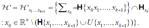
Observe that for every plane Σ_x0 we have that x₀∈Σ_x0.

Now we need to show that the dimension of the set = x₁...,x_k+1 is equal to n and that each plane in is of dimension k.

To prove that observe that since is parameterized via the set ℝⁿ \(H{x₁,…,x_k+1}∪U{ x₁,…,x_k+1}) which is of dimension n we have that dimH0≤n. In order to prove that we will prove that for any two different points x’ and x’’ the planes Σ_x’ and Σ_x’’ are different. Indeed, since Σx’ ⊂Hx’ it follows that its closest point to the origin is x’ and in the same way x’’ is the closest point of Σ_x’’ to the origin. Hence, if Σ_x’ =Σ_x’’ it follows that both x’ and x’’ are the closest points of a k plane to the origin and they are both different. This obviously leads to a contradiction.

To show that for each x₀∈ℝⁿ the plane Σx₀ is of dimension k we first observe that since x₀∈Σ_x0 then Σ_x0 is a nonempty intersection of a hyperplane and a k+1 plane in ℝⁿ. Hence, dimΣx₀ is equal to k or k+1 where the later case occurs when H{ x₀,…,x_k+1} is contained in H_x0. This will imply in particular that

x₁,…,x_k+1∈H_x0 and thus

⟨x₀–x₁,x₀⟩=…=⟨ x₀– x_k+1,x₀⟩=0

which is a contradiction to the assumption that x∉{x₁,…,x_k+1}. Now, for every function f, defined in ℝⁿ, which decays to zero fast enough at infinity, our aim is to recover f from which is now restricted to the smaller set and thus our problem is well posed. For this we have the following result.

Theorem 2.1: Let f be a function in C^∞ (ℝⁿ) (the space of infinitely differentiable functions in ℝⁿ) which satifises the decaying condition f(x)=o(|x|^–N) for some N>k+1. Then, f can be recovered from its k dimensional Radon transform restricted to the set of k dimensional planes.

Proof: From here and after we will assume, without loss of generality, that {x_k+1–x₁,…x_k+1–x_k} is an orthonormal set. Since if this is not the case then by equation [2.1] it follows that there exists an orthonormal set of vectors {y₁,…,y_k} such that

span{y₁,…,y_k}=span{x_k+1–x₁,…x_k+1–x_k}.

Hence, if we denote x_i*= x_k+1–y_i then it is easily verified that

H{x₁,…,x_k,x_k+1}=H{x₁ *,…,x_k *, x_k+1}.

Hence, for the set {x₁ *,…,x_k *, x_k+1} we obtain the same set of k planes, i.e.,

and we also have that {x_k+1–x₁ *,… x_k+1– x_k *} is an orthonormal set.

The proof of Theorem 2.1 is divided into 5 parts.

In the first part we find necessary and sucffient conditions on a point x₀ in ℝⁿ\(H{x₁,…,x_k+1}∪U{x₁,…,x_k+1}) so that the k plane Σ_x0 is contained in a given k+1 plane Σ’.

In the second part we define a special subset of k+1 planes.

In the third part we find, with the help of the first part, necessary and sufficient conditions on a point x₀ in ℝⁿ\(H{x₁,…,x_k+1}∪U{x₁,…,x_k+1}) for the k plane Σ_x0 to be contained in a given k+1 plane in .

In the fourth part we show that the union of all the k+1 planes in is the whole space ℝⁿ.

Lastly, in the fifth part we show that the k planes in , which are contained in a given k+1 plane Σ’ in , are in fact all the k planes in Σ’ and thus the function f, in Theorem 2.1, can be recovered on Σ’. Since, by the fourth part, the union of the k+1 planes in is the whole space ℝⁿ it follows that f can be recovered in ℝⁿ. This will finish the proof of Theorem 2.1.

Finding conditions on the point x₀ so that the k plane Σ_x0 is contained in a given k+1 plane Σ’: For x₀∈ℝⁿ \(H{x₁,…,x_k+1}∪U{x₁,…,x_k+1}) observe that the k plane Σ_x0 in can be parameterized as follows

From the above parametrization we obtained for Σ_x0 it follows that for every ω∈S^n-1 and c∈ℝ the k plane Σ_x0 is contained in the hyperplane ⟨x,ω⟩=c if and only if the following two conditions are satifised

i. ⟨x,ω⟩=c,

ii. There exists an index 1≤i≤k+1 such that ⟨x_i–x₀,x₀⟩≠0 and

⟨x_i–x₀,x₀⟩⟨x_j–x₀,ω⟩=⟨x_j–x₀, x₀⟩⟨x_i–x₀, ω⟩ for j=1,…,i–1,i+1,…,k+1.

Now, for a given k+1 plane Σ’ we would like to nd necessary and sufficient conditions on x₀ so that the k plane Σ_x0 is contained in Σ’. Let us assume that Σ’ is given by the following system of equations

⟨x, ω_i⟩=μ_i,i=1,…,n–k–1

where ω₁,…ω_n–k–1 form an orthonormal set and where μ₁,…,μ_n–k–1∈ℝ. From the above analysis it follows that the k plane Σ_x0 is contained in a k+1 plane Σ’, given by the intersection of all hyperplanes given by [2.2], if and only if the following two conditions are satifised

(i*) ⟨x₀,ω_i⟩= μ_i,i=1,…,n–k–1,

(ii*) For every 1≤i’≤n–k–1there exists an index 1≤i≤k+1 such that ⟨x_i–x₀, x₀⟩≠0 and such that

⟨x_i–x₀,x₀⟩⟨x_j–x₀, ω_i’⟩=⟨x_j–x₀,x₀⟩⟨x_i–x₀, ω_i’⟩ for j=1,…,i–1,i+1,…,k+1.

Defining the set of k+1 planes: Now, let us look only on k+1 planes given as the intersection of the n–k–1 hyperplanes given by [2.2] where ω₁,…,ω_n–k–1 satisfy

⟨x_k+1– x_i,ω_j⟩=0,i=1,…k,j=1,n–k–1 [2.3]

and where the parameters μ₁,…,μ_n–k–1 are then given by the following equations

μ_j=⟨x_k+1,ω_j⟩(=⟨ xi,ω_j⟩,i=1,…,k),j=1,…,n–k–1 [2.4]

Denote this family of k+1 planes by . That is,

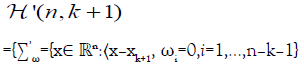
:ω=(ω₁,…,ω_n–k–1), where ω_i,i=1,…,n–k–1 form an orthonormal set in S^n-1 and belong to span{x_k+1–x₁– x₁,… x_k+1–x_k}┴}.

Finding conditions on the point x₀ so that the k plane Σ_x0 is contained in the k+1 planeΣ^’_ω in : Let us take a k+1 plane Σ^’ _ω in . Then, for a k plane Σ_x0 to be contained in Σ^’ _ω the point x₀ in ℝⁿ\(H{x₁,…, x_k+1}∪U{x₁,…,x_k+1}) needs to satisfy only condition (i*) since then condition (ii*) is also satisfied. Indeed, since x₀∉U{x₁,…, x_k+1} there exists an index i such that ⟨x₁– x₀, x₀⟩≠0. Using the fact that for Σ^’ _ω we have, from equation [2.3], that ⟨x_i,ω_i⟩=⟨x_k+1,ω_i’⟩, it follows that

⟨x_i–x₀,ω_i’⟩=⟨x_i,ω i’⟩–⟨x₀,ω i’⟩=⟨x_k+1,ω i’⟩– μ i’=0

where in the second passage we used condition (i*) and in the last passage we used equation [2.4]. In the same way we can show that ⟨x_j–x₀,ω i’⟩=0 and thus condition (ii*) is obviously satisfied.

Thus, it follows that the k plane Σ_x0 is contained in the k+1 plane Σ^’ _ω in if and only if

⟨x₀,ω i⟩=⟨x_k+1,ω i⟩,i=1,…,n–k–1.

The k+1 planes in cover the whole space ℝⁿ: Our aim is to reconstruct f on every k+1 plane Σ^’ _ω in (n,k+1). If this can be done then f can be recovered on the whole of ℝⁿ. Indeed, we only need to show that for every z₀∈ℝⁿ there exists a k+1 plane Σ^{`</sup><sub>w</sub> in such that z<sub>0</sub>∈ Σ<sup>`}_w. That is, we need to find n–k–1 orthonormal vectors ω₁,…,ω_n–k–1 such that each of them is orthogonal to x_k+1– x₁,…,x_k+1–x_k and such that the following equations are satisfied

⟨z₀, ω i⟩=⟨x_k+1, ω_i⟩,i=1,…,n–k–1

That is, the orthonormal system ω₁,…,ω_n–k–1 needs to be orthogonal to . Since is spanned by k+1 vectors it follows that and thus. Thus, we can find an orthonormal system ω₁,… ,ω_n–k–1 which is in . The corresponding parameters μ₁,…,μ_n–k–1 are then uniquely determined by equation [2.4].

Recovering f on each k+1 plane in : Let us take a k+1 plane Σ^’ _ω in and show how f can be recovered on Σ^’ _ω. As we previously mentioned, we can assume that {x_k+1–x₁,…,x_k+1–x_k} is an orthonormal set. Hence, since the vectors ω₁,…,ω_n–k–1 also form an orthonormal set then from equation [2.3] it follows that {x_k+1–x₁,…, x_k+1–x_k,ω₁,…,ω_n–k–1} is an orthonormal set. Thus, there exists a rotation A such that A(x_k+1–x₁)=e₁,…, A(x_k+1–x_k)= e_k, Aω₁=e_k+2,…,Aω_n–k–1= en.

Let us choose a point x₀∈ℝⁿ\(H{x₁,…,x_k+1}∪U{x₁,…,x_k+1}) such that the k plane Σ_x0 is contained in the k+1 plane Σ^’ _ω. If we denote x^’ ₀=Ax₀, x^’ _k+1=Ax k+1 then condition [2.5] is equivalent to

⟨x’,ei+k+1⟩=⟨x^’ _k+1, ei+k+1⟩,i=1,…,n–k–1. [2.6]

The assumption that x₀ is not in the unique k plane which passes through x₁,…,x_k+1 is equivalent to the assumption that rank {x_k+1– x₀,x_k+1– x₁,…,x_k+1– x_k}=k+1 or equivalently that rank {x^’ _k+1– x^’ ₀,e1,…,ek}=k+1 and from equation [2.6] this is equivalent to x^’ ₀,k+1≠ x^’ _k+1,k+1. The assumption that x₀∉U{x₁,…,x_k+1} is equivalent to the assumption that there exists an index 1≤i≤k+1 such that ⟨x_i–x₀,x₀⟩≠0 or equivalently that ⟨x’ i–x^’ ₀,x^’ ₀⟩≠0 where we denote x’ i=Axi.

Hence, the k plane AΣ_x0 is contained in the k+1 plane AΣ^’ _ω if and only if x^’ ₀=Ax₀ has the form

x^’ ₀=(u,u₀), u₀=( x^’ _k+1.k+2,…,x^’ _k+1,n), u∈ ℝ^k+1 [2.7]

and which satisfies the following condition

u k+1≠x’k+1,k+1, ∃i,1≤i≤k+1,⟨x’ i– x^’ ₀, x^’ ₀⟩≠0

or equivalently the condition

(iii) u k+1≠ x’k+1,k+1∃i,1≤i≤k+1,⟨x’ i–(u,u₀),(u,u₀)⟩ ≠0

Let us recall again that the k+1 plane Σ^’ _ω is given by the system of equations

⟨x,ω_i⟩=⟨ x_k+1,ω_i⟩,i=1,…,n–k–1

or equivalently by the system of equations

⟨Ax,e_k+i+1⟩=⟨ x’k+1, e_k+i+1⟩, i=1,…,n–k–1.

Hence, the k+1 plane AΣ^’ _ω is given by

AΣ^’ _ω={(u,u₀):u∈ℝ ^k+1,u₀=(x^’_k+1,k+2,…, x’_k+1,n)}

and for this plane we define its origin to be the point (0,u₀). Now, we claim that for each point x^’₀ which is of the form [2.7] and satisfies condition (iii) the closest point of the k plane AΣ_x0 to the origin in AΣ^’ _ω is obtained at x^’₀. Indeed, the closest point of Σ_x0 to the origin is x₀ (since Σ_x0 ⊂Hx₀) and thus the closest point of AΣ_x0 to the origin is x^’ ₀=Ax₀. Now, if there exists a point x”∈ AΣ_x0 ⊂AΣ^’ _ω whose distance to the origin (0,u₀) in AΣ^’ _ω is smaller than that of x^’₀ then we can assume that x^’ ₀=(u,u₀), x’’ 0=(u’’,u₀),u, u’’∈ℝ^k+1 and where |u’’|<|u|. This will imply that |x’’ 0|< |x^’ ₀|an so x’’ 0 is a point in AΣ_x0 whose distance to the origin in ℝⁿ is smaller than that of x^’ ₀. This is obviously a contradiction.

Hence, for a point x₀ such that x^’ ₀= Ax₀ is of the form (u,u₀), where u satisfies condition (iii), we have that AΣ_x0 ⊂ AΣ^’ _ω and that its closest point to the origin in AΣ^’ _ω is obtained at x^’ ₀. This means that if we project the k+1 plane Σ^’ _ω= ℝ^k+1 ×{u₀} to ℝ^k+1 then the closest point, of the projection of AΣ^’ _ω, to the origin 0 in ℝ^k+1 is obtained at the point u.

Thus, it follows that the projection of AΣ_x0 to ℝ^k+1 is the following k dimensional hyperplane

Π _u={⟨ x’–u,u⟩=0: x’∈ℝ^k+1}. [2.8]

Now, the restriction that the point u must satisfy condition (iii) can be omitted since the set of points u which do not satisfy this condition is of co dimension 1 in ℝ^k+1. Thus, by passing to limits when preforming integration we can obviously obtain the integrals on any hyperplane of the form [2.8]. Thus, we can assume that u∈ℝ^k+1. Hence, if u= rσ where r≥0, σ∈S^k then the k plane IIu is given by

Π^’ _r,σ={⟨ x’,σ⟩= r: x’∈ℝ^k+1}.

Observe that every k dimensional hyperplane in ℝ ^k+1can be written as Π^’ _r,σ for some fixed r≥0,σ ∈S^k. Every function in C∞ o(ℝ ^k+1) which decays to zero faster than |x|–N, N>k+1, at infinity can be recovered from its classical Radon transform (see 7, Chap. 1.3, Theorem 3.1) which integrates the function on every k dimensional hyperplane in ℝ ^k+1. From our assumption on the function f it follows that the restriction of g = foA^–1 to the k+1 plane AΣ^’ _ω satisfies these conditions and thus it can be recovered on this plane. Equivalently, this means that f can be recovered on Σ^’ _ω. Thus, Theorem 2.1 is proved.

The case of integration on lines in ℝ³ with a fixed distance from a given point

For r>0, a point p in ℝ³ and a compactly supported continuous function f, defined on ℝ³, we consider the following problem. Suppose that the integrals of f are given on each line whose distance from the point p is equal to r and we would like to recover f from this family Π of lines. Since the intersection of the interior of the sphere S’=S(p,r) with any line in Π is empty then obviously f cannot be recovered inside S’ and thus we can assume that each function in question vanishes inside S’. Without loss of generality we can assume that p=0; r=1. That is, our family Π consists of all the lines which are tangent to the unit sphere S² and our aim is to recover a continuous compactly supported function, which vanishes inside S², given its integrals on each line in Π. Since S² is of dimension two and since, for each point p∈ S², the family of lines which are tangent to S² and pass through p is one dimensional it follows that dim Π=3. Hence, our problem is well-posed.

Observe that for a point x∈ℝ³, satisfying |x| ≥1, the family of all lines which are tangent to the unit sphere S² and pass through x is a cone with the apex at x which is tangent to S² where the tangency set is a circle on S². Let us denote by Cx Ʌthe above considered cone and denote by Ʌ the family of all such cones which are obtained by taking points x∈ℝ³ satisfying |x|≥1. Observe that if x=λe3 where λ≥1 then the family Ʌ can be parameterized as follows

Ʌ={A^–1C _λe3: A∈SO(2), λ≥1}

where SO(2) denotes the group of rotations in ℝ³. For every λ≥1 the cone C _λe3 can be parameterized as follows

Now, let f be a continuous function, defined in ℝ³, with compact support. Then, our data consists of the following integrals

Remark 2.2: Observe that with the parametrization [2.9] of the cone C _λe3 we have that its innitesimal area measure is given by . However, in our case the expression dSx given in equation [2.10] is chosen such that (i.e., the term |t| is omitted). We can choose dSx in this way since for every λ ≥1 we know the factorization of C _λe3 into lines passing through its apex. Each such line, given by the parametrization [2.9],

where the parameter φ is fixed, has infinitesimal length measure given by λdt. Thus, we can just integrate on this family of lines with respect to φ with the infinitesimal angular measure dφ .

Our aim is to recover f from the family of integrals given by equation [2.10]. The inversion formula is given in Theorem 2.3 below. Before formulating and proving Theorem 2.3 we introduce some notations and definitions.

For every integer m ≥0 denote by the Gegenbauer polynomial of order ½ and degree m.

Let T_A,A∈SO(2) be the quasi-regular representation of the group So(2). That is, for a function g∈L² (S²) the operator T acts on g by T_A(g)=goA^–1.

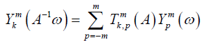
Let be an orthonormal complete system of spherical harmonics in S² and let be the components of the representation matrix of T with respect to this family of spherical harmonics. That is

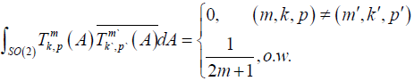
The functions satisfy the following orthogonality relations (see 8, Chap. 1.5.2).

Now we can formulate Theorem 2.3.

Theorem 2.3: Let f be a continuous function, dened in ℝ³, which has compact support and vanishes inside S² and let

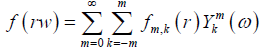
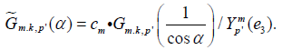
be the expansion of f into spherical harmonics. Denote

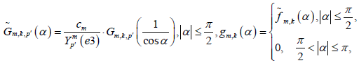
where

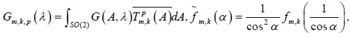
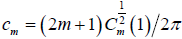and where is defined on the whole interval [–π,π] by defining

.

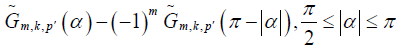Then, for the following Fourier expansions on the interval [–π,π]

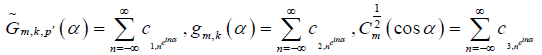
we have that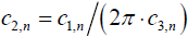

Remark 2.4:

In Theorem 2.3 the parameter p’,|p’|≤m can be any parameter which satisfies . Also, observe that by Theorem 2.3 we can recover the function gm,k and thus we can also recover the function e which is equivalent of recovering f_m,k on [1,∞). Since, by our assumption, f vanishes inside S² it follows that f_m,k vanishes in [0,1] and thus we can extract f_m,k on the whole line ℝ. Hence, since we can obtain f_m,k for every m≥0.|k|≤m then obviously the function f can be recovered.

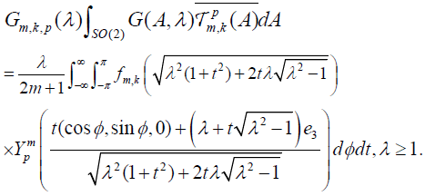
Proof of Theorem 2.3: For every A∈SO (2) we have

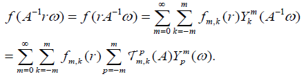
Using the orthogonality relations for the family of functions on SO(2) we have that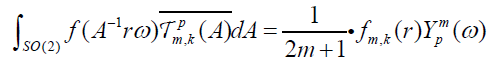. Hence, we obtained that 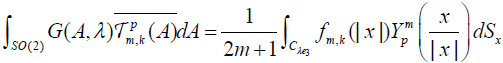where λ≥1 and pj m. Using the parametrization [2.9] of the cone C _λe3 we have

[2.11]

Let α be a point in the interval [–π,π) such that

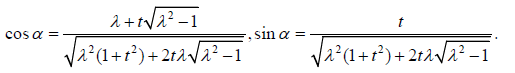
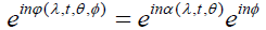
Every spherical harmonic in S² satisfies the following identity (see for example [7-9]

[2.12]

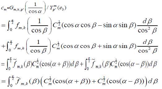
Where ψ ∈S². Hence, using equations [2.11]-[2.12] and the definition of the parameter cm we have

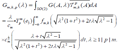[2.13]

Now, observe that there exists an integer p satisfying |p|≤m such that . Otherwise we can just choose a spherical harmonic Y^m of degree m and choose a point ω₀∈S² such that Y^m (ω₀)≠0. Then, if A is a rotation such that Aω₀=e3 then K(ω)=Y^m (A^–1ω) will also be a spherical harmonic of degree m such that K(e₃)≠0. Now, since K can be expanded into spherical harmonics from the family ,|p|≤m then if for every |p|≤m then we will also have K(e₃)=0 which is a contradiction.

Let us choose p’,|p’|≤m such that . Then, from equation [2.13] we have

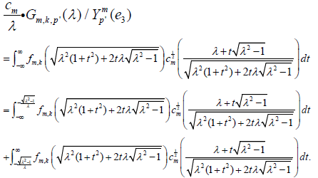[2.14]

Observe that the function 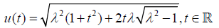is injective on the intervals ( and [).

Hence, we can make the following change of variables

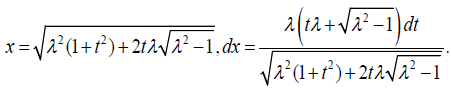[2.15]

Extracting the variable t from equation [2.15] we have

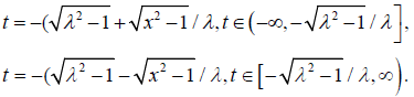
In both cases we have 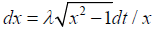. Thus

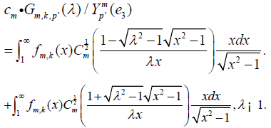
Denoting λ’=1/λ and making the change of variables x=1=x’ we have

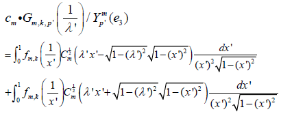[2.17]

where 0≤λ’≤1. Observe that both integrals in equation [2.17] converge since for every m≥0,|k|≤m the function f_m,k vanishes at infinity (since, by assumption, f is compactly supported). Hence, there is no singularity near x’= 0.

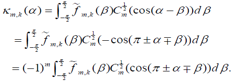
Let us denote λ’=cosα,0≤α≤ π/2 and make the change of variables x’=cosβ. Then, from equation [2.17] we have

where we define

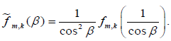
Observe that is an even function dened on –π=2≤β≤π/2. Since the sum of the Gegenbauer polynomials in the integral [2.18] is an even function of β it follows that

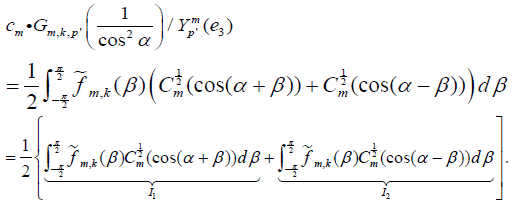Since is an even function of it follows easily that I₁ = I₂. Thus,

[2.19]

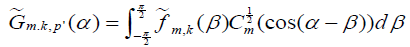
where we denote

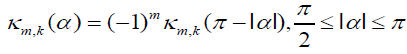
Observe that the right hand side of equation [2.19] is given for 0≤α≤π/2, but using the change of variables β↦–β and using the evenness of it follows that the right hand side of equation [2.19] is an even function of α. Hence, can be extended, as an even function of α to the interval [–π/2,π/2]. The right hand side of equation [2.19] is defined for all α∈[–π,π] and if we denote it by then we have that

.

Indeed, let α satisfy π/2≤|α|≤π, then we have

Hence, in case where π/2≤α≤π then we choose the sign and then by making the change of variables β↦– β and using the evenness of we have . In case where –π≤α≤–π/2 then we choose the sign and then we can prove in the exact same way that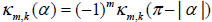. Hence, if we extend the function to the larger domain [–π,π] by defining 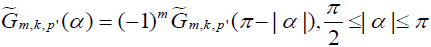then equation [19] is valid for all α in [–π,π]. Let us define the function gm,k as follows

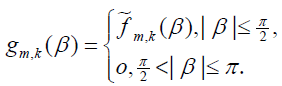
Then, from equation [2.19] we have

[2.20]

Assume now that and gm,k are defined on the whole line ℝ by taking their 2π periodic extensions. Bearing in mind that the convolution h3 of two 2π periodic functions h1 and h2 is defined by 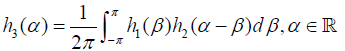and that the convolution theorem for this type of functions asserts that if then , Theorem 2.3 is obtained from equation [2.20] and by using the expansions of and into their corresponding Fourier series.

The case of integration on lines in ℝ³ with equal distances from two given points

Let x and y be two distinct points in ℝ³ and consider the family Π of all lines which have equal distances from these points. Without loss of generality we can assume that x=e3,y=–e3. In this case it can be easily observed that Π is the set of all lines whose distance to the origin is obtained at their intersection point with the XY plane, when considering lines which are not contained in this plane, and also all the lines which are contained in the XY plane. In other words, for each point in the XY plane we consider the unique hyperplane Hp which passes through p and whose normal is in the direction of and then we take all the lines which pass through p and are contained in Hp. Since the family of hyperplanes Hp where is two dimensional and the set of all lines which pass through p and are contained in Hp is one dimensional it follows that dim Π=3 (in case where then we can take all the lines which pass through p).

Our aim in this section is to recover a continuous function f, defined in ℝ³, in case where we are given the integrals of f on the set of all lines in Π. Since dim Π=3 our problem is well posed. In order to guarantee that inversion formulas are obtainable, when considering integration on lines in Π, we must restrict our family of functions since any function which is radial with respect to the variable and is odd with respect to the variable x₃ produces no signals. However, if we assume that f is compactly supported in the half space x₃ > 0 then we can obtain an inversion formula as will be proved in Theorem 2.5 below.

Before formulating Theorem 2.5 we will need first to parameterize the family of lines Π and introduce the Mellin transform. Observe that since Π is invariant with respect to rotations which leave the vector e3 fixed it follows that it is enough to parameterize the subset of lines in Π which are parallel to the YZ plane (and then we take rotations of these lines with respect to the Z axis to obtain the whole set Π). If a line l in this subset has a distance λ≥0 from the origin and its projection to the YZ plane forms an angle θ,– π/2≤θ<π/2 with the Y axis then l has the following parametrization

Hence, we obtain the following parametrization

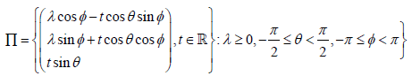[2.21]

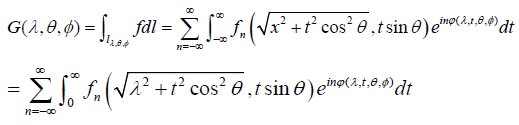
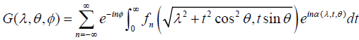
for the family Π. If the function G=G(λ,θ,∅) is defined by

[2.22]

where ℝ⁺ denotes the ray [0,∞) and dl is the infinitesimal length measure on the line l, then our aim is to express the function f via G.

For a function F, defined in ℝ⁺, define the Mellin transform F of F by

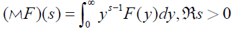[2.23]

where it should be noted that the above integral might not converge for every complex number s satisfying ℜ>0 . For the Mellin transform we have the following inversion formula (see 10, Chap. 8.2)

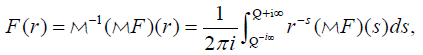[2.24]

where Q>0 . The inversion formula [2.24] is valid for many types of functions whereas in our case we will justify its application in the particular case where F is continuous and has compact support (see Lemma 2.7). We will also need the following scaling property

if 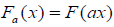where a > 0 then

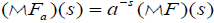[2.25]

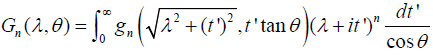
see [10], Chap. 8.3). Formula [2.25] is valid in any domain for which the Mellin transforms of F and Fa exist and hence we will have to justify the existence of these transforms, in the corresponding domain, each time this scaling property is used [11]. If F is a function of two variables then we denote by the Melling transform of F with respect to its i^th variable. Finally, for every integer n and complex numbers ζ,ξ define the following integral

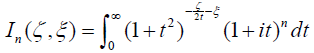[2.26]

where I_n might not converge for every ζ and ξ. Now we can formulate Theorem 2.5.

Theorem 2.5: Let f be a continuous function, defined in ℝ³, which is compactly supported in the half space x3>0 and let G be defined as in [2.22] [12]. Let

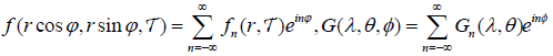[2.27]

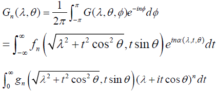
be the Fourier expansions of f and G respectively in the variables ϕ and ∅. Define

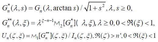
where n ' = max(0, n +1), then

[2.28]

Remark 2.6: When using the Mellin inversion formula [2.24] in equation [2.28] then when using , for which integration is taken with respect to the variable ζ, the point Q must be taken from the ray [n’,∞] whereas when using , for which integration is taken with respect to the variable ξ, the point Q must be taken from the interval [0,1] [13]. This is to ensure that integration is taken over the domain of definition of for which the integral n I converges.

Proof of Theorem 2.5: In the domain of definition of the function G let us assume for now that the variable θ is restricted to the interval [0,π/2] [14]. Then, integrating f on the line l_λ,θ,Ø with its parametrization given in equation [2.21] and using the expansion [2.27] of f we obtain

[2.29]

where

and where in the last passage of equation [2.29] we used the fact that f is supported on the half-space x3 > 0 and that sinθ≥0 if 0≤θ≤π/2. The following relation

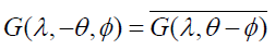
can be easily checked and thus, assuming that λ≥0 and –π≤∅<π, negative values of θ do not give any new information on f and hence we will assume from now on that θ is given only in the interval [0,π/2]. Now, define the variable so that

then

we have

Hence,

and thus we have

from which we obtain that

[2.30]

where we denote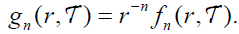

Making the change of variables t’=t cosθ in the right hand side of equation [2.30] we obtain that

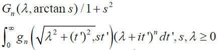
If we denote s=tanθ then since 0≤θ≤π/2 it follows that s≥0 and, since in this domain of θ, we can write

.

Hence, if we define by the following relation 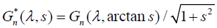and then take the Mellin transform with respect to the variable s on both sides of the last equation we obtain that

[2.31]

Where λ ≥∣ 0,0 < ℜ(ξ ) <1. The application of the Mellin scaling property [2.25] is justified here since for every λ,t’≥0 the function

is compactly supported in s [since f is compactly supported in ℝ³ and thus obviously gn is compactly supported with respect to both variables r and ] and thus, using Lemma 2.7 [see the end of this section] [15], it follows that its Mellin transform exists for every ℜξ > 0 . The restriction that 0 <ℜ(ξ ) <1 is to ensure that the integral I_n, as defined by equation [2.26], which will appear later in the computation, converges.

Making the change of variables t’=λt in the right hand side of equation [2.31] yields

[2.32]

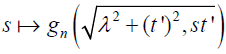
Denoting

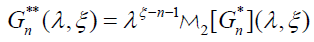
and then taking the Mellin transform, with respect to the variable λ, on the integral in the right hand side of equation [2.32] and on yields

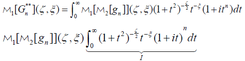
where the application of the Mellin scaling property, for the variable λ, can be justified in the exact same way as we previously did for the variable s. Observe that since R(ζ ) > n' and 0 <R(ξ ) <1 then the integral I = I_n (ζ ξ) converges. Indeed, at t→0+ the integrand behaves like t^–ξ and for t→∞ if n≤–1 then n I obviously converges while for n≥0 the integrand behaves like 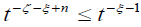and I_n converges also for this case. Dividing both sides of the last equation by I_n (ζ ξ) and then taking the inverse Mellin transform in both variables ζ and ξ we can obtain Theorem 2.5.

The application of the Mellin inversion formula [2.24] for g_n and for can be justified since these functions have compact support in the corresponding variables on which the Mellin transforms are applied [gn is finitely supported in its second variable and is finitely supported in its first variable] [16]. Hence, the justification of these inversion formulas are now an easy consequence of Lemma 2.7.

Lemma 2.7: F :ℝ⁺ →ℝ be a continuous function with compact support. Then, the Mellin transform of F exists on each line where c > 0 and one can use the Mellin inversion formula [2.24] for Q=c in order to reconstruct F.

Proof: Let us evaluate the Mellin transform of F on the line l_c. Assume that F is supported inside the interval [0, a ] where a > 0 , then

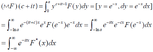
Where

Since c > 0 it follows that F* is in L₁ℝ and thus its Fourier transform exists in ℝ which is equivalent to the fact that the Mellin transform of F exists on the line l_c. Inverting F from its Mellin transform [2.23] is equivalent to inverting F* from its Fourier transform and since F is continuous it follows that F* is also continuous and since it is also in L₁ℝ then it is well known that one can use the Fourier inversion formula in order to recover F* . This finishes the proof of Lemma 2.7.

REFERENCES

1. Radon J. On the Determination of Functions by Their Integral Values ​​of Certain Manifolds. Ber. Verh. Sachs. Akad. Leipzig. Math. Nat. Cl. 1917;69:262-277.
2. Cormack AM. Representation of a function by its line integrals, with some radiological applications. J Appl  Phys. 1963;34:2722-2727.
3. Deans SR. The Radon transform and some of its applications. Dover Publ. Inc., Mineola, New York. 2007.
4. Rubin B, Wang Y. New inversion formulas for Radon transforms on affine Grassmannians, arXiv:1610.02109.
5. Palamodov VP. Reconstruction from Integral Data. Monographs and Research Notes in Mathematics. CRC Press, Boca Raton. 2016.
6. Palamodov VP. Reconstructive integral geometry. Monographs in Mathematics. Birkhauser, Basel. 2004.
7. Natterer F. The Mathematics of Computerized Tomography. Wiley, New York. 1986.
8. Volchkov VV. Integral Geometry and Convolution Equations. Kluwer Academic, Dordrecht. 2003.
9. Agranovsky M, Volchkov VV, Zalcman LA. Conical uniqueness sets for the spherical Radon transform. Bulletin of the London Mathematical Society. 1999;31:231-236.
10. Dambaru B, Debnath L. Integral Transforms and Their Applications. CRC Press, New York. 2007.
11. Gel'fand IM, Gindikin SG, Graev MI. Selected topics in integral geometry, Translations of Mathematical Monographs. AMS, Providence, RI. 2003.
12. Helgason S, Integral geometry and Radon transform. Springer, New York-Dordrecht Heidelberg-London. 2011.
13. Helgason S. The Radon Transform, Birkhauser, Basel. 1980.
14. Mader P. About the representation of point functions in Euclidean space by plane integrals. Mathematical J. 1927;26:646-652.
15. Rubin B. On the Funk-Radon-Helgason inversion method in integral geometry, Cont Math. 2013;599:175-198.
16. Rubin B. Reconstruction of functions from their integrals over k dimensional planes, Israel J Math. 2004;141:93-117.