


 +447723598358

Principles of prime numbers - Part IV - Twin prime & Polignac conjectures – Conservation of gaps
Received: 29-Jul-2026, Manuscript No. PULJPAM-26-7757; Editor assigned: 31-Jul-2026, Pre QC No. PULJPAM-26-7757 (PQ); Reviewed: 14-Aug-2026 QC No. PULJPAM-26-7757; Revised: 27-Aug-2026, Manuscript No. PULJPAM-26-7757 (R); Published: 03-Sep-2026, DOI: 10.37532/2752-8081.2026.10(1).1-20
This open-access article is distributed under the terms of the Creative Commons Attribution Non-Commercial License (CC BY-NC) (http://creativecommons.org/licenses/by-nc/4.0/), which permits reuse, distribution and reproduction of the article, provided that the original work is properly cited and the reuse is restricted to noncommercial purposes. For commercial reuse, contact reprints@pulsus.com
Abstract
The prior papers “Principles of Prime Numbers - Part I - New Definition of Prime Numbers with ModNt Number System & Induction”, “Principles of Prime Numbers - Part II - Anatomy of Sppn & Rppn Tables with Conversion from mod10 to modNt Number System” and “Principles of Prime Numbers - Part III - Sppn & Rppn Table Parameters with Advanced Topics and Twin Prime Conjecture” must be read to put this paper into perspective. Those papers are a summary of three books “Calculate Primes” (2007), “Principles of Prime Numbers – Volume I” (2010) and “Breaking RSA Codes” (2014). Another peer reviewed paper can be included in the list of prior papers “New Definition of Prime Numbers with Sppn Tables and Proofs by Induction”.
In the prior books and papers, the concept of direct calculation of prime numbers was presented using the McCanney Generator Function and a sole boundary condition. It showed that the prime numbers constitute a complete number system modNt based on sequential prime products Sppn with visual representation in the form of “Sppn and Rppn tables”, creating the basis for proofs by induction for the Twin Prime Conjecture and other problems. The groups of prime numbers form algebraic groups. Groups of prime numbers generate larger groups beginning with Peano’s Postulates. The new mathematical system has properties of closure, completeness, reciprocity, symmetry and generates the wave equations “combn ” that predict all future primes to infinity. Each prime number or series of prime numbers has a unique ancestry. This is demonstrated in the digits of the modNt number system. Likewise, each prime or group of primes has an infinite number of descendants. Composite numbers that are relatively prime to the values of Sppn are important in the development of real primes, twin primes and larger groupings of real primes. Without these relative primes, the process would not generate all real primes and would not be complete. Prime numbers belong to families with ancestors, descendants as well as siblings.
Keywords
Prime numbers; Twin prime conjecture; Polignac conjecture; Calculate primes
Introduction
Prior papers Parts I, II and III [1-3] presented many concepts with basic examples including the basis for the proof of the Twin Prime & Polignac Conjectures. They demonstrated the more than exponential growth of the twin prime only Sppn tables discovering real twin primes. The formulae which generate future Sppn tables show why this occurs. The current paper Part IV presents a proof for the Twin Prime Conjecture and arrives at the conclusion that there is an infinite number of twin primes. It advances that there is another way of looking at this infinity based on the work on transfinite numbers by Georg Cantor. This new view states that “every relative twin prime pair generates an infinite number of future real twin primes”. Thus, starting at any point in any Sppn twin prime only table, every relative twin prime pair will generate an infinite number of real twin primes and thus is not a simple countable infinity. Relative primes are needed to generate the entire complete list of true primes, true twin primes or prime pairs of any gap size.
Also formalized is the concept that extends to gaps of 4 and larger showing that there is an infinite number of subsequent gap sizes and refines the concept of “Conservation of Gaps” introduced in prior papers. It is demonstrated that once a gap of size k is encountered (k=2, 4, 6 …), it continues to generate relative prime gaps of the same size in all future Sppn Tables and therefore will continue to generate real prime pairs of this gap size to infinity (presenting a solution to the Polignac Conjecture of which the Twin Prime Conjecture is a special case).
It is a result of the fact that only one “white cell” (products pn × pj where pn is the nth prime number and pi is the list of combn-1 elements) per column does not transfer to the subsequent table Sppn+1. It also gives understanding to the Goldbach Conjecture which will be the topic of the next Part V paper, showing that the criteria for failure of the Goldbach Conjecture can be understood and tested using induction. As with the Twin Prime Conjecture, it depends on the well-organized Sppn tables building subsequent tables Sppn+1 from prior tables. The problem is understood in pieces. It also shows that the Goldbach solutions come in families and the solutions are related to ancestors and descendants as are all primes. The combn-1 formulae are generalized to predict twin primes with repeating wavelength of Sppn-1 to infinity. The ratio of (√Sppn)/Sppn-1 is shown to be the basis for understanding the growth of twin primes as well as primes in general as demonstrated in prior papers.
Before presenting the proposed solution to the Twin Prime Conjecture, the discussion will review concepts built in prior papers. This will be followed by the proposed proof of the Twin Prime Conjecture concentrating on the following:
• “Conservation of Prime Gaps”
• importance of the expression (√Sppn)/Sppn-1 (the E=mc2 of prime numbers)
• Rppn tables
• the concept of “duplicate products”
• the effects of gap size on the final solution
Materials and Methods
Review and summary of prior papers
Use the following two diagrams of “Anatomy of an Sppn table” and “Anatomy of Rppn table” to help interpret the text below (Figures 1 and 2).
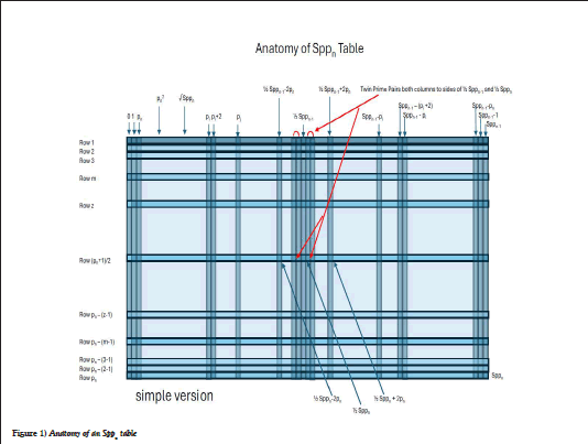
Figure 1) Anatomy of an Sppn table
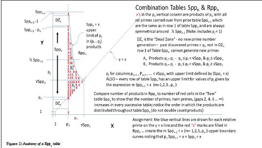
Figure 2) Anatomy of a Rppn table
All elements of row 1 of an Sppn table are defined as the combn-1 of wavelength Sppn-1 which repeats to infinity and contains all future relative primes including all real prime numbers using the expression=mSppn-1 + combn-1 (m=1, 2, 3 …). All relative primes in table Sppn that are not real primes are eliminated using the Rppn table which is the mapping of all the products pi × pj where pi are all numbers from row 1 such that pi=pn, pn+1, pn+2, … pmax < √Sppn and pj are all elements of row 1 such that pj=1 and pi ≤ pj ≤ (Sppn ÷ pi). The first series of these products have a special purpose (pn × pj) and are labeled “white cells” since they are not relatively prime to Sppn. Duplicate products arise and there is a process for eliminating duplicate products. Each future table has a larger percentage of duplicate products, the effect of which will be explained. It is the Rppn table that is used to determine the number of real primes in each Sppn table by eliminating composite numbers.
A subsequent table Sppn+1 is formed by first stringing rows 1 through pn of table Sppn in sequence (after removing the “white cells”) to form row 1 of table Sppn+1. Complete rows 2 through pn+1 by adding multiples of Sppn to the numbers in row 1. It will be shown that every subsequent Sppn+1 table has more primes, twin primes, prime pairs of gap k, or gap patterns than in the prior table. There will not only by more, but more than exponentially more in each subsequent Sppn+1 table. It is the essential piece of the puzzle needed to prove the Twin Prime Conjecture. The ability to divide the direct calculation of prime numbers into groups (the Sppn tables) allows for generalized equations to be built which leads to the proof by induction.
The Twin Prime Conjecture is a special case of the general case defined by the conservation of gaps which states that every pair of relative primes of gap k in each table Sppn will produce an infinite number of future prime pairs of gap k. As the tables are developed, the future combs are modifications of prior combs by reducing the number of elements and therefore puts an upper limit on the counting function. This is an important development over prior counting functions in that it: 1) Predicts exactly where to find primes, twin primes or prime pairs of any gap size or gap pattern and 2) Sets the upper limit on the location of primes (the prior methods only could give a local average leaving the possibility of rogue gaps or rogue primes) and 3) It creates a family structure of the primes having ancestors, descendants, cousins and distant relatives. This is why twin primes continue to occur no matter how far out the number line you go and no matter how far apart the prime numbers become. With each subsequent Sppn table, the predicting equation (combn-1) is refined to be more precise than the prior table.
A new number system results directly from the McCanney Generator Function called Nature’s Number System or modNt. As opposed to mod10 or other modulo number systems, it uses the Sppn values 2, 6, 30, 210, 2310, … for digits (rather than for example 10, 100, 1000 … in mod10 system). It is the natural number system of prime numbers. It is one of major discoveries of this series of papers first presented in the 2007 book “Calculate Primes” [4]. It was shown in prior papers that the modulo M number systems were a hindrance to understanding prime numbers. When used in conjunction with the Sppn tables, prime numbers are noted by sequences based on their modNt ancestry. Every number has an ancestral path going back to the alpha prime pα=0. Every digit of the modNt number represents a generation ancestor. The ancestral path going back to the alpha prime pα=0 involves removing modNt digits requiring no calculations, unlike mod10 numbers all of which show no ancestral heritage or patterns, and for which extensive calculations are required for each one. In the Sppn table using the modNt number system, the value of a given cell derives its higher order digit from the left column and lower order digits from the value of the cell at the top row 1 of the Sppn table. For this reason, all the values of a given Sppn table need not be filled in since all you need is the value of the left column and top row (unlike mod10 numbers which require extensive calculations and which are unrelated by any patterns).
The Sppn tables contain only real and relatively prime numbers and form a complete isolated number system. Since the cells are colored red, they are termed as “red cell only”. The red cell only Sppn table can be further reduced to tables specific to certain gap sizes such as the twin prime only tables which has its own combn-1 predictive equation. This comb is the same as the comb for the complete red cell only table (which contains all relative primes including all real primes from pn to Sppn) but with only the relative twin primes of row 1 and their respective columns included. When working with the twin prime only table (or any table containing only row 1 relative prime pairs of a given gap size k), all real twin prime pairs from pn to Sppn are contained in the columns of this table. All future twin primes (or pairs of primes of gap k) are predicted by the combn-1 equation, being directly calculated in groups by addition only. This is the fundamental concept of the new definition of primes numbers and directly calculating prime numbers (no long division or other numbers are necessary).
The structure of “white cells” is a major discovery. It has been established that there is one and only one white cell in a given column in the Sppn table, therefore any relative prime pair of gap k that exists in row 1 of any Sppn table will have pn-2 pairs with gap k in its columns to carry forward to form row 1 of the subsequent table Sppn+1 . By induction, this process continues to infinity, guaranteeing the propagation of all gap sizes once they are formed in the parent Sppn table. The other part of the solution shows that there is: 1) a greater than exponential increase in red cells in each subsequent table, 2) while there is an exponentially diminishing number of composite numbers (non-primes) products of pi × pj in each subsequent table. The result is a more than exponential growth of primes, twin primes or prime pairs of gap k in each subsequent table. Examples were given in the previous papers of this series. It cannot be stressed enough, the importance of the concept that relative primes are as much a prime number as real prime numbers in a given Sppn table and are instrumental in generating real primes in future tables. These are not counted as real primes; they are only used in the generation process of calculating real primes. This is one of the pieces of the puzzle that has been missing in the understanding of prime numbers.
Once a gap of length k has been generated, it will continue to generate gaps of length k in all future tables to infinity. A comb equation can be written from any of the tables to predict all descendant gaps, and all future gaps k will have ancestry leading back to the original prime pair which will be reflected in the digits of the modNt number. There is an aspect to the concept of “Conservation of Gaps” in that, if a large gap occurs in the list of prime numbers, then there will be small gaps nearby to compensate for the large gap. Look at the prime number table to verify this is true. Likewise, if there is a small gap in a region or series of small gaps, there will be a large gap to balance. The principle of “Conservation of Gaps” is a formulated as a theorem. This is because there is a fixed number of products pi × pj that “cancel cells” in a given Sppn table (produce non-primes), so if they tend to cluster in one area of the Sppn table (creating a large gap), then that leaves fewer products to cancel primes in nearby areas of the same table. This is observed in the scope of analyzing the Sppn tables.
It was also established in the prior papers that if a large gap occurs in a given area of the prime number table, the large gap does NOT carry to future Sppn tables or affect the future distribution of gaps in any way, since the large gap is a local event in the Rppn product table caused by a clustering of products pi × pj. Since there is a set number of products that identify composite numbers, this means that near this clustering there will be a lack composite numbers (causing the gaps of smaller sizes). These two statements may seem to be contradictory but are not. This is because the real prime gaps themselves do not carry to generate future tables, but the entire red table (all rows and columns) carry forward to the next Sppn+1 table except for the evenly (and symmetrically) distributed white cells for which one and only one occurs in the columns of the prior table to build row 1 of the subsequent table. An example is the largely out of place gap 34 between 1327 and 1361. It is due to a clustering of products in the Sppn table but does not carry to future Sppn+1 tables. As prime numbers get larger, the max gaps have relatively smaller deviations from the average gap of the region. This is another result of the combn-1 equations that predict all prime numbers preventing “rogue gaps”. The following is a summary of progression of tables from n=α (pα=0) to n= 6 (p6=13) developed in prior papers of this series to review the process of building tables.
Review of prior work – Gap k=2 (Twin primes): Relative twin prime gaps carrying to future tables and generate real twin primes. Look in the Sppn tables below and follow a relative twin prime pair into subsequent tables. For this example, chose (17, 19) found in row 1 of table n=4 with p4=7 and Spp4=210 (Figures 3 and 4). Looking down the columns below 17 and 19, locate the generated pair (167,169*). 169 is marked with a star (*) denoting a relative prime. 167 and 169 are generated by adding multiples of Sppn-1=30 to 17 and 19. 169 has its lowest prime factor 13 which is larger than p4=7. It is relatively prime to 210=2 × 3 × 5 × 7. 169 is as much of a prime number in this table as any real prime. Although it is not itself a prime number, it is needed to generate future real prime numbers and therefore real twin prime in this table as any real prime. Although it is not itself a prime number, it is needed to generate future real prime numbers and therefore real twin prime pairs. It is this understanding of the roll of relative prime numbers in the generation of real prime numbers that has been missing in the standard definition and view of prime numbers. See all the twin primes (relative and real) generated in row 2 to pn=7 in table Spp4 below. Figure 3 shows the sequence of Sppn tables from the n=α (alpha) table and Peano’s Postulates to table n=4. Figure 4 shows the n=4 table with all prime and non-prime numbers color coded. Figure 5 removes all other non-relative prime columns showing the progression to “red cell only” table n=4. Figure 6 shows only the twin prime columns in the “red twin prime only” table (one could also select a gap k=4 table that would create a gap 4 only table) [4]. These are the ancestors of all future twin primes using the McCanney Generator Function which is visualized in the Sppn tables.
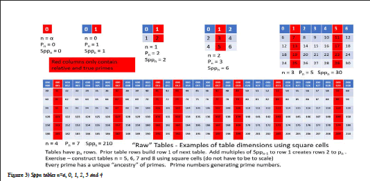
Figure 3) Sppn tables n=a, 0, 1, 2, 3 and 4
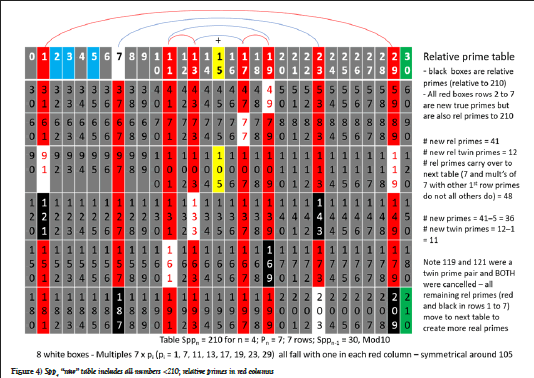
Figure 4) Spp4 “raw” table includes all numbers <210; relative primes in red columns
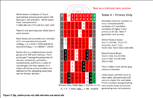
Figure 5) Spp4 relative primes only table with white and colored cells
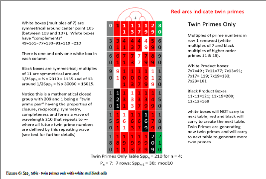
Figure 6) Spp4 table - twin primes only with white and black cells
The n=4 “red cell only” Figure 5 is shown above. All the prime numbers (relative and real) are found in the red columns, being generated by the prior table group of prime numbers. This is an autonomous set of numbers closed under addition. This is the basis of “Calculate Primes”. It is a self-contained mathematical system of prime numbers (prime numbers generating prime numbers in groups using only the operation of addition).
Use the standard method to create table Spp5 from table Spp4 (see red only Spp5 table Figure 7 below). Find (167,169*) in row 1 of table Spp5 and see all the generated relative prime pairs of gap k=2 (twin prime pairs) in the columns below (many will be discovered to be real twin primes). Then find all the other twin prime pairs in row 1 and all of the generated twin prime pairs in the columns below these (locate twin primes using the red arcs above the pairs). Gap sizes are identified by color coded arcs connecting adjacent columns. After including the white cells, for each relative twin prime pair in row 1, there will be (p5–2)=11–2=9 relative twin prime pairs that proceed to row 1 of the next table Spp6. This is a multiplication of 9 and this number increases in the next table by another factor of (p6–2)=13- 2=11. Be sure to include the twin prime pair (1, 29) (Figure 6) which in the columns below generates (29,31), (59,61), (149,151), (179,181) and (209,1) which will generate more twin primes in the subsequent table. As explained in prior papers of this series, addition is closed as in an Abelian group (the rational for grouping 29 with 1 and 209 with 1). Follow these to row 1 of the following table. Select the gap 4 pairs and do the same as they propagate into subsequent tables.
Below is the series of Spp5 tables generated from the n=4 tables above. Figure 7 below is the “raw” Spp5 red cell only table using mod10 numbers with no white cells or other colored cells noted. It contains all real primes and cells whose values are relatively prime to Spp5=2310. It is closed in that all factors of composite numbers in this table are contained in row 1. It is also closed under group addition. It is complete in that all numbers that are not relatively prime to Spp5 are not found in this table and all numbers that are relatively prime to 2310 (including all real primes) are found in this table. There is reciprocity such that all cells of the prior table Spp4 can be calculated from all cells in this table. There are numerous symmetries including but not limited to 1) row 1 symmetry around midpoint ½ Spp4=105, 2) symmetry all cells around midpoint of table Spp5=2310/2=1155 and 3) there is symmetry in comb5-1 when added to and subtracted from Spp5-1=210 to predict all future relative prime numbers to infinity. Figure 8 is the definition of modNt number system to 510,509. Figure 9 is the same Spp5 table but converted to modNt numbering. Figure 10 is the same n=5 table with white and black colored cells (products of 13). Figure 11 is table n=5 with blue columns marked to note columns that have no twin primes (to be removed in creating the Figure 12). Figure 12 is the twin prime red cell only table. Figure 13 is the twin prime only table with white cells marked. Figure 14 is the same table with white cells and all other products from the Rpp5 table applied (black cells). Figure 15 is the isolated rows of table Spp5 ready to be placed to form row 1 of table Spp6. These tables were developed in prior papers with the intent of using them for the final proof of the Twin Prime Conjecture using induction.
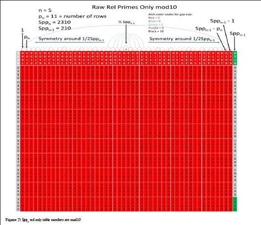
Figure 7) Spp5 red only table numbers are mod10
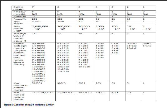
Figure 8) Definition of modNt numbers to 510509
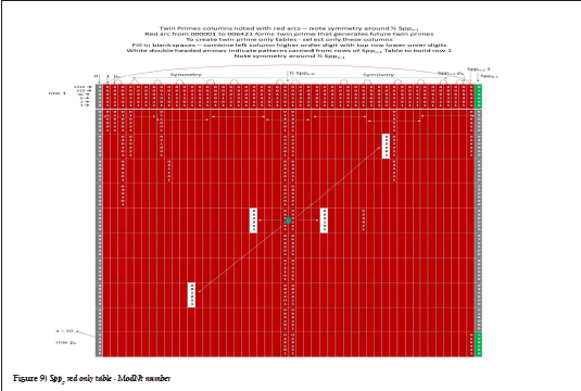
Figure 9) Spp5 red only table - ModNt number
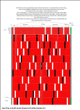
Figure 10) Spp5 red only table with white cells (products of 11) and black cells (products of 13)
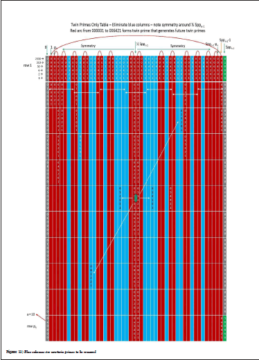
Figure 11) Blue columns are non-twin primes to be removed
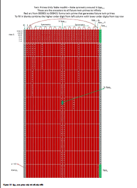
Figure 12) Spp5 twin prime only red cell only table
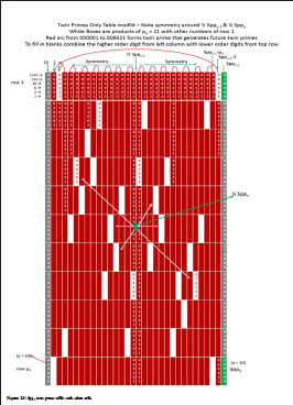
Figure 13) Spp5 twin prime table with white cells
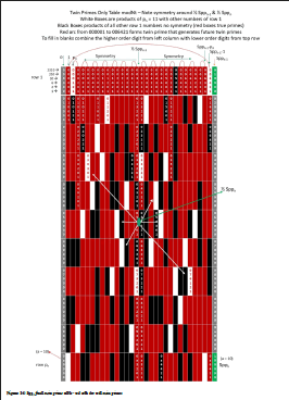
Figure 14) Spp5 final twin prime table - red cells are real twin primes
At this point we are going to transition to modNt number system to determine the real twin primes. The definition of modNt numbers up to 510,509 is given in Figure 8. In following the pair (167,169*), the modNt equivalent values are (5221, 5301) found in row 1 of Figure 14.
The conversion of (167,169*) to modNt values is as follows:
• 5221 modNt = 5 × 30 + 2 × 6 + 2 x 2 + 1 × 1=167 mod10
• 5301 modNt = 5 × 30 + 3 × 6 + 0 x 2 + 1 × 1=169 mod10
The red cell only twin prime table with white cells Spp5 (Figure 13) is the table used to generate the next twin prime only table Spp6 by stringing the rows 1 to p5=11 in sequence to build row 1 of the twin prime only table n=6. From this point forward the twin prime calculations are autonomous. They are a subset of the prime number red tables. Only the white cells (the cells not relatively prime to Spp5=2310) do not transfer to create row 1 of the next table. Notice the symmetry of both the red and white cells around the ½ point of row 1 and ½ point of the table (the green oval in the center of the table). For example, if you took the white cell pattern and rotated it 180 degrees it would show the exact same pattern. This table building process is the visualization of the McCanney Generator Function and its boundary condition. Figure 14 is the same table with all products (white and black cells) noted [5]. All the red cells that remain are true prime numbers. If both members of a twin prime remain then it is a true twin prime. Twin primes are discovered in groups by direct calculations from prior groups of relative primes. This was the original intent of the book titled “Calculate Primes”.
Now follow all newly generated pairs (including the black cells because they are relatively prime) to the next table n=6 with p6=13. Put into sequence rows 1 through p5=11 of table n=5 in Figure 15 below (remove white cells before creating row 1 of table n=6) where more relative twin primes are generated, all of which will move to row 1 of the n=7 table to generate many more. In table n=7 with p7=17, p6=13 will move into the Dead Zone DZ7 and although (167,169) it will not directly generate more twin primes, all of the relative twin prime pairs that it generated will continue to branch out and this process continues to infinity (if you doubt this continue the process as long as you like). Rather than carry out this Promethean or otherwise Sisyphean operation, this can be formalized into a proof by induction where it is shown that gap k=2 will generate more relative prime pairs of gap k=2 (twin primes) in each subsequent table continuing to infinity. The following is the formalization showing growth from one table Sppn to the subsequent table Sppn+1 and proposed proof of the Twin Prime Conjecture that is both based on the new mathematical system and visualized in the Sppn and Rppn tables.
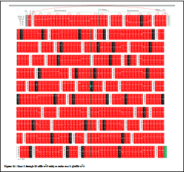
Figure 15) Rows 1 through 11 table n=5 ready to create row 1 of table n=6
Conservation of gaps – The key (√Sppn)/Sppn-1 – Rppn tables
Solution the twin prime conjecture: The topic of conservation of gaps was initiated in the prior papers of this series (especially Part III). The best way to present this is in the visualization of the Sppn tables (the visual representation of the McCanney Generator Function) demonstrating the importance of (√Sppn)/Sppn-1 and Rppn tables as they generate groups of real primes, real twin primes and prime pairs of gap k. Although some of this may sound repetitive, this is the formal (text book) presentation.
First, we will formalize how a subsequent table Sppn+1 is created from a previous table Sppn as developed in prior papers, but with a few more details that illustrate how the subsequent Sppn+1 table produces a greater than exponential increase in discovering real primes (and real twin primes or prime pairs of gap k). Prior papers have constructed Sppn tables up to n=6 for p6=13 and Spp6=30,030. This was to demonstrate the principles of table generation before formalizing with generalized equations using “red cell only tables”. The “red cell only” tables contain only real primes and composite numbers that are relatively prime to Sppn. It is a self-contained system.
The process has properties of closure. All factors of the composite numbers are contained in row 1 of a given Sppn table. The Sppn tables are closed under the operation of addition in Abelian groups and this carries from one table to the next when generating subsequent tables. The process has completeness. All relative prime numbers (relative to Sppn) which includes all real primes are contained in the table from pn up to the value of the sequential prime product Sppn. The tables exhibit property of reciprocity because the process is reversable; with the modNt number system every digit represents the ancestry of the prime number or pair of prime numbers back to the prior table and eventually to the original ancestor pair. The system exhibits many symmetries. These include:
• Symmetry of red cells around the midpoint of row 1=½ Sppn-1
• Row 1 symmetry carries to create symmetry for both red and white cells of the entire Sppn table around the center point of the table=½ Sppn
• The combn-1 equation of table Sppn,which predicts all prime numbers to infinity, is symmetrical in that it predicts prime numbers when added to and subtracted from the sequential prime product Sppn-1 from the definition of the McCanney generator function.
• There are additional symmetries not discussed in this paper (e.g. around multiples of Sppn)
Lastly, the system exhibits wave nature with the combn-1 (all members of row 1 of table Sppn) added to multiples of the wavelength Sppn-1=mSppn-1 + combn-1 (m=1, 2, 3, … ∞). This explains the seeming patterns that emerge then fade in the prime number table that are interpreted as “random” or “pseudorandom”. It is the beating of these wave equations that creates this illusion. These patterns center around multiples of wavelength Sppn-1. Pick any multiple of any Sppn-1 value and look to the right and left to see these patterns (taking the difference between prime numbers and these numbers). Also visible are regions like dead zones to the right and left of these numbers. Specific comb equations (subsets of the comb equations) predict for example all twin primes or all gaps of a given value k.
This is a result of a redefinition of prime numbers with a single boundary condition [6]. The new definition states that the only numbers that can be prime are those resulting from adding relative prime numbers to sequential prime products, with the single boundary condition that all numbers less than the square of pn are prime. The entire point is to create new tools which allow proof by induction in addition to creating a new number system based solely on primes. The result is to define a new mathematical structure of primes for primes and by primes with the foundation in Peano’s Postulates. The system shows the importance of relatively prime composite numbers in this process.
The process of generating table Sppn+1 starts with table Sppn which has pn rows. The “red cell only” Sppn+1 table is constructed from the prior table Sppn by the following:
1) Mark the “white cells” in table Sppn
• The “white cells” are the products pn × pj (subscript “j” from the Rppn table) where pn is the nth prime number associated with table Sppn and pj being the elements of combn-1 which are all the red cells (real and relative primes of row 1 of table Sppn).
• There is one and only one white cell in each column of table Sppn, therefore the total number of white cells is the same as the number of columns of table Sppn uses the variable Mn
2) Place rows 1 through pn of red cell only table Sppn in succession to form row 1 of table Sppn+1 with the first cell value=0 and the last cell value=Sppn. The rest of the cells of column 0 and Sppn (rows 2 to pn) do not carry over, and the white cells do not carry over since they are not relatively prime to Sppn and will no longer generate future relative primes. The resulting Sppn+1 row 1 values are:
• [ 0, 1, pn+1, pn+2, … , (Sppn – pn+2), (Sppn – pn+1), (Sppn – 1), Sppn]
• This is called combn of table Sppn+1 (note the subscripts) and has Mn+1 values which are symmetrical around the midpoint 1/2 Sppn. This symmetry carries from one table to the next. When added to multiples of the wavelength Sppn, combn provides the equation that predicts all prime numbers to infinity. When compared to the prior combn-1 (row 1 of the prior table), combn refines (reduces) the possible values and therefore becomes more accurate at predicting real prime numbers. These equations provide a monotonically decreasing prediction of all prime numbers (assuring there are no rogue primes or gaps) and predicts precisely where to find real primes, twin primes and prime patterns. The combn contains both real and all composite numbers that are relatively prime to Sppn giving the predictive equation for all prime numbers as follows:
• mSppn + [ 0, 1, pn+1, pn+2, … , (Sppn – pn+2), (Sppn – pn+1), (Sppn – 1), Sppn] where m=1, 2, 3, … ∞.
• This also provides a test or primality when using the modNt number system (all future primes must end in one of these sequences modNt … if a future number does not end with one of these sequences, then it is not prime).
• Per the McCanney generator function on which these tables are based, 1 and (Sppn-1) are always relatively prime to Sppn and therefore will always carry to the next table row 1 (these are a primary source of twin prime pairs in every table and could be used to prove the Twin Prime Conjecture on its own).
• The prime number pn related to table Sppn is retired to the dead zone DZn+1 of Sppn+1 as it will not generate any future primes (although all the primes and relative primes that it generated will continue to generate primes until they eventually enter the dead zone of their respective tables).
3) The numerical values of red cells of rows 2 to pn+1 in the columns of table Sppn+1 are calculated by adding multiples of Sppn to the values in row 1 of table Sppn+1 proceeding up to row pn+1. kn is the gap between pn+1 and pn (kn=pn+1 – pn). There are various opinions of the definition of gaps but this one works well with this system. The total number of cells in row 1 of table Sppn+1 is equal to the total number of cells in row 1 of table Sppn (Mn) multiplied by (pn-1). The “- 1” accounts for the white cells that do not carry from the prior table to form row 1. This is the basis for the generalized equation where the dimensions and other properties of a given table can be calculated without creating all the intermediate tables. Table Sppn has pn rows and Mn columns so there are Mn × pn red cells total (before removing white cells). Table Sppn+1 has pn+1=pn + kn rows and Mn+1 = Mn × (pn-1) columns so there are Mn+1 × pn+1 red cells. All patterns of prime numbers derived from all prior tables are maintained and visible in each table. That is why patterns seem to come and go in the prime number tables only to be replaced by other patterns. These patterns center around the values of Sppn and its multiples where n=α, 0, 1, 2, 3 … ∞, giving the illusion of “random” or “pseudo random” patterns. Instead they are like waves of different wave lengths on an infinite ocean beating against each other.
4) To generate the subsequent table Sppn+2 return to the top and begin again by selecting the white cells of table Sppn+1.
5) The final step is to determine the number of real primes or real twin primes generated in the process. There are two methods used. Notation below uses the perspective of table Sppn generating table Sppn+1 while determining the number of primes in table Sppn+1. First understand that the table is closed under multiplication. This means that if a number in this table has factors (is not prime), those factors are contained in row 1 [7,8]. Row 1 (combn) contains all relative primes (composite and real primes) from the prior table.
• The first method of selecting true prime numbers is the Boundary Condition of the McCanney Generator Function which is also the new definition of prime numbers. It states that all red cells of table Sppn+1 whose values are less than p2n+1 are prime. This is because there can be no products in this region, therefore it is a region that is a “safe zone”. Since the prior table Sppn discovered all real primes up to p2n the criteria are stated such that all comb members between p2n and p2n+1 are newly discovered primes. This can be used to prove that there are an infinite number of individual prime numbers but is not useful in proving the Polignac or Twin Prime Conjectures.
• The second method of identifying prime numbers in table Sppn+1 is used in the proof of the Twin Prime Conjecture and can be seen in the tables below (derived from prior papers). The red only Sppn+1 table contains all relative primes between pn+1 and Sppn+1 (all composite numbers whose factors are relatively prime to Sppn+1 and real primes). The use of these tools is what has been missing from analysis of prime numbers, leading to the view of prime numbers in manageable pieces where one table generates the next allowing proof by induction. As noted above, the red cell only tables are closed under multiplication. This means that all the composite numbers in the table can be identified by multiplying elements of row 1 with other elements of row 1. All red cells not identified by this process will be prime. The Rppn+1 table constitutes a mapping of all products pi × pj of elements of row 1. The growth of the number of discovered true primes (and twin primes) with increasing counting integer “n” shows this progression. The solution is to generalize this progression of building a new Sppn+1 table from a prior table Sppn to prove that each subsequent Sppn+1 table has exponentially more primes and twin primes than the prior table. Since this is the general case and not dependent of specific numbers, the proof will proceed by induction.
• Review of Rppn+1 table generation (developed in prior papers of this series). Key values in the Rppn+1 table are √Sppn+1 (located in row 1) and the ratio √Sppn+1/Sppn. √Sppn+1 is the maximum value of a member of row 1 of table Sppn+1 that can be multiplied by itself and fit inside the Sppn+1 table. The products pi x pj from row 1 are pi=pn+1, pn+2, pn+3, … , pmax < √Sppn+1 and pj are all elements of row 1 such that pj= 1 and pi ≤ pj ≤ (Sppn+1 ÷ pi). The first series of these products have a special purpose (pn+1 × pj) and are labeled “white cells” since they are not relatively prime to Sppn+1. The products are written in sequence as follows (pi subscript “i” is from the x axis and pj (subscript “j”) is from the y axis of table Rppn+1 noting the order of subscripts to prevent duplication):
a) pn+1 × [1, pn+1, pn+2, pn+3, … , (Sppn – pn+3), (Sppn – pn+2), (Sppn – pn+1), (Sppn – 1)]
• Products of pn+1 with all elements of row 1 including pn+1 × 1 and pn+1 × (Sppn – 1))
• Note the symmetry around midpoint of row 1=½ Sppn
• This creates vertical line of red x’s above pn+1 on Rppn+1 graph (as an exercise draw in the red x’s on the Rppn+1 graph below)
b) pn+2 × [pn+2, pn+3, pn+4, … , pmax < (Sppn+1/pn+2)]
• Note the upper limit pmax of the second term pj is limited by Sppn+1/pi
• This creates second vertical line on Rppn+1 graph above pn+2
c) pn+3 × [pn+3, pn+4, pn+5, … , pmax < (Sppn+1/pn+3)]
d) Continue until pimax < √Sppn+1
e) Pimax × pimax=p2 imax
This creates the final red x on Rppn+1 graph less than √Sppn+1
See the progression of tables below from Rppn to Rppn+1 (Figure 16). The Rppn+1 graph contains all the products (composite numbers) that can then be mapped back into the Sppn+1 table to identify composite numbers (leaving only true primes). If one can show that the progression from one Sppn table to the subsequent table Sppn+1 produces not only more, but exponentially more true primes (and twin primes), then the original claim will be proven that each relative prime (and each relative twin prime) produces an infinite number of future real primes (and twin primes).
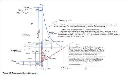
Figure 16) Progression of Rppn tables n to n+1
Tables 1 and 2 show the parameter results up to table n=11 (p11=31) with the most notable found in Table 2 the fifth column and right hand column. This shows the growth of twin prime pairs discovered in Sppn tables. The generalization of this growth using induction is the basis for the proof of the Twin Prime Conjecture. It is both mathematical and visual (thanks to the Sppn tables). You do not have to generate all the Sppn tables to infinity since generalized equations are about to be demonstrated to show that each subsequent table generates more real twin primes than the prior table and by induction, gives the result that “every relative twin prime generates an infinite number of real twin primes”. The proof involves the understanding gained from the Rppn tables and the expression √Sppn/Sppn-1.
| n | Pn mod10 (also number of rows in Sppn table) | Pn modNt | Sppn Mod10 vs. modNt modNt=10n (greater than exponential growth) | vSppn mod10 upper limit relative prime pi of row 1 such that pi² |
vVSppn)/ Spp n-1 |
Number columns red only table (also number of elements in combn-1)=# red cells Sppn-1 table less white cells in n-1 table | Total number red only cells=Sppn Table= prior column × Pn | Prior column /Sppn= fraction red cells vs. Sppn |
| a | 0 | 0 | N/A | N/A | N/A | N/A | N/A | N/A |
| 0 | 1 | 1 | 1/100 | 1.0 | N/A | N/A | N/A | N/A |
| 1 | 2 | 10 | 2/101 | 1.4 | 1.414 | 0 | 2 | 1.000 |
| 2 | 3 | 11 | 6/102 | 2.4 | 1.225 | 1 | 3 | 0.500 |
| 3 | 5 | 21 | 30/103 | 5.4 | 0.913 | 2 | 10 | 0.333 |
| 4 | 7 | 101 | 210/104 | 14.4 | 0.483 | 8 | 56 | 0.267 |
| 5 | 11 | 121 | 2310/105 | 48.0 | 0.228 | 48 | 528 | 0.229 |
| 6 | 13 | 201 | 30030/106 | 173.2 | 0.075 | 480 | 6240 | 0.208 |
| 7 | 17 | 221 | 510510/107 | 714.5 | 0.024 | 5760 | 97920 | 0.192 |
| 8 | 19 | 301 | 9699690/108 | 3114.4 | 0.0061 | 92160 | 1751040 | 0.181 |
| 9 | 23 | 321 | 223092870/109 | 14936.2 | 0.0015 | 1658880 | 38154240 | 0.171 |
| 10 | 29 | 421 | 6469693230/1010 | 80434.4 | 0.00036 | 36495360 | 1058365440 | 0.164 |
| 11 | 31 | 1001 | 200560490130/1011 | 447839.8 | 0.000069 | 1021870080 | 31677972480 | 0.158 |
Table 1: Parameters for Sppn tables to n=11
| n | Pn | Gap n kn-1 = Pn-Pn-1 | Number of new primes discovered pn-1²<pi<pn |
Total number new primes discovered Sppn table using Rppn table (rows 2 to Pn) | Number of column pairs - twin prime only table (also 2x this value = number of elements in twin prime combn-1) | Total number relative twin prime pairs in Sppn table (red cells only) = prior column × Pn | Number of new twin primes discovered pn-12<pi<pn |
Total Number new twin primes discovered Sppn Table using Rppn Table (rows 2 to Pn) |
| ? | 0 | N/A | N/A | 1 | 0 | 0 | 0 | 0 |
| 0 | 1 | 1 | N/A | 1 | 0 | 0 | 0 | 0 |
| 1 | 2 | 1 | N/A | 1 | 0 | 0 | 1 | 0 |
| 2 | 3 | 1 | 2 | 2 | 0 | 0 | 1 | 2 |
| 3 | 5 | 2 | 5 | 7 | 1 | 5 | 2 | 3 |
| 4 | 7 | 2 | 6 | 36 | 3 | 21 | 2 | 10 |
| 5 | 11 | 4 | 15 | 297 | 15 | 165 | 4 | 55 |
| 6 | 13 | 2 | 9 | 2903 | 135 | 1755 | 2 | 398 |
| 7 | 17 | 4 | 22 | 39083 | 1485 | 25245 | 7 | 4168 |
| 8 | 19 | 2 | 11 | 603698 | 22275 | 423225 | 2 | 52817 |
| 9 | 23 | 4 | 27 | 11637502 | 378675 | 8709525 | 4 | TBD |
| 10 | 29 | 6 | 47 | TBD | 7952175 | 230613075 | 8 | TBD |
| 11 | 31 | 2 | 16 | TBD | 214708725 | 6655970475 | 2 | TBD |
Table 2: Parameters for Sppn tables to n=11
Take the ratio of primes discovered by Rppn (column 5 Table 2 above), noting that the number of prime numbers discovered are from rows 2 to pn in their respective Sppn tables. This is because the real primes in row 1 had already been reported on the prior table. The ratios (from n=1 to n=9) are as follows: 2/1=2, 7/2=3.5, 36/7=5.14, 297/36=8.25, 2903/297=9.77, 39083/2903=13.86, 603698/39083=15.45 and 11637502/603698=19.28 … note the more than exponential increase. Take the difference between the increases and note that the gap 4 ratios have larger increases than gap 2 ratios. This is because the subsequent Sppn+1 table has more rows at the bottom of its table than the prior table (there are more red cells relative to the number of products that locate composite numbers). As tables grow with larger gaps, this is a factor that further increases the growth of discovered primes (general equations will be developed below).
Follow the same procedure finding the ratios of twin primes discovered by Rppn. They are as follows: 3/2=1.5, 10/3=3.33, 55/10=5.5, 398/55=7.24, 4168/398=10.47, 52817/4168=12.67 … note the more than exponential increase. This progression continues to infinity. In the n=8 table the process is discovering 603,609 real primes and 52,817 twin primes.
Next see the successive values of √Sppn/Sppn-1 starting with n=1 to n=11. The proportion (percentage) of products in each successive Rppn table is greatly reduced while the table size (number of red cells) is greatly increasing. Each subsequent table has more than exponentially more primes and twin primes than the prior table. These numerical examples do not constitute proof but simply illustrate the mathematical relationship between tables as they grow. The proof relies on the generalization of this process showing that this growth continues to infinity.
The following is a detailed example (Figure 17) showing the importance of (√Sppn)/Sppn-1 and comparing it to this ratio for the subsequent Sppn+1 table (√Sppn+1)/Sppn, noting that this number decreases rapidly with increasing values of the counting integer “n”. The following is a visual representation of the generation of table Spp6 from table Spp5 also showing generalized formulae. This table is the key to understanding the growth from one table to the next such that there are exponentially more newly discovered primes in each table.
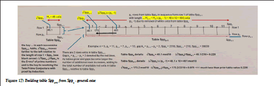
Figure 17) Building table Sppn+1 from Sppn - general case
In Figure 17, the dimensions of table Sppn are Mn=48 cells (columns) and pn=11 rows. After removing white cells from table Sppn, the rows from 1 to pn are moved in sequence to form row 1 of table Sppn+1. Note in the drawing this is being compared in table Sppn+1 to Mn+1=Mn × (pn – 1)=48 × 10=480 cells (columns) but only pn rows (see red dashed lines connecting the two tables). This is done on purpose to compare the number of products pi × pj of each table with the same number of rows in both tables, leaving the 2 additional rows at the bottom of table Sppn+1 (noted by the two solid red lines) to be added in later. To get a proportional number of products as table Sppn in the Rppn+1 table (identifying composite numbers of table Sppn+1), one would use the cut off value of √Sppn × (pn -1)=481. However, the table Sppn+1 cutoff value is √Sppn+1=173.2 with the ratio √Sppn+1/Sppn=173.2/210=0.75 (compared to 0.228 for table Sppn). The generalized equation going from table Sppn to Sppn+1 for the ratio R between √Sppn+1 and √Sppn × (pn – 1) is as follows:
As n the counting integer increases and the gap kn becomes small relative to the value of pn, the right side increases as the square of the left side. This proves that for all cases of creating subsequent tables, the cutoff value √Sppn+1 is much smaller than the prior table. The same result occurs comparing the ratio between (√Sppn+1)/Sppn and √Sppn/Sppn-1 with the similar result √pn+1 R pn. This explains the increase in growth of primes, twin primes and prime pairs of gap k in successive Sppn tables.
Relative to the originator table Sppn there are proportionately fewer products to create composite numbers in table Sppn+1. This is why the ratio √Sppn/ Sppn-1 is called the E=mc2 of prime numbers. Understanding its effect on table generation holds the key to the growth of primes, twin primes and prime pairs of any gap k.
There are other effects that further cause a larger disparity between the number of products pi × pj in the Rppn+1 table from the prior table and therefore add additional real primes discovered as each new table is created. The first is the addition of the extra kn rows at the bottom of table Sppn+1 due to the gap between pn and pn+1. The generalized equation is as follows with specific example n=5 to n=6:
General equation=Mn+1 × kn=Mn × (pn -1) × kn
Example Figure 17 table Spp6=480 × 2=960 additional red cells. As the gap sizes grow and the length of the tables increases, this adds a significant number of red cells and therefore real primes. These were not included in the original analysis which used the same number of rows=pn in both tables, so these extra rows are now added to the number of red cells (and therefore real primes) left after removing composite numbers generated in the Rppn+1 table. This effect alone would be sufficient to prove the Twin Prime Conjecture.
The second effect is the fact that each subsequent Rppn table has more duplicate products than the prior table. This indirectly adds more red cells to the final count of discovered real primes because these products are not producing new unique composite numbers that would cancel potential real primes. Figure 18 above shows an example of table with duplicate products (color coded). The proof would proceed without this effect so is not stressed (it is a subject for future more esoteric studies).
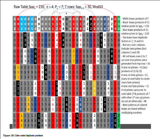
Figure 18) Color coded duplicate products
If at this point anyone has doubts about the process, please continue building tables and filling in the values until you are convinced that this will repeat to infinity. Then realize the generalized equations are sufficient to prove the result that:
• Every relative prime (relatively prime to Sppn) will generate an infinite number of real primes.
• Every relative twin prime pair (relatively prime to Sppn) will generate an infinite number of real twin prime pairs.
QED
Goldbach conjecture -proofs by induction: Presented here are concepts that help in understanding the basis for Goldbach Conjecture solutions. It has been pointed out in prior papers that the reason there are local maximums of the Goldbach pairs at values of Sppn (or multiples of these values) is because of the symmetry of the Sppn tables around the half point ½ Sppn. The white cells eliminate relative primes symmetrically around the ½ point and therefore leaves all other red cells in the table. Every remaining red cell has a compliment cell that adds to Sppn. The local GB maximums are a direct result of the symmetry of primes in the Sppn table. As you move away from Sppn the “alignments” become fewer and many times the adjacent alignment creates far fewer Goldbach pairs. To find the number of Goldbach pairs for the number Sppn–2, combine all the prior solutions for Sppn and find only those that are the second member of a twin prime pair. Combine these with the other number and their sum will be Sppn – 2. To complete the process, take any two elements with real primes that add to a given even number and note their columns. In these columns there will be more prime pairs that add to that same number.
Looking at row 1 of the Sppn table, find two primes that add to an even number less than the max value in row 1 which is Sppn-1. Follow the two primes moving down in their respective columns and the numbers generated in these columns are Goldbach solutions to the row 1 plus a multiple of Sppn-1. This creates families of solutions just as the twin primes generate other twin primes. These families are identifiable in the patterns of GB solutions as they fan out above the x axis. This is only introduced here and is a topic for one of the future papers in this series. The question is asked: “what would it take to break the Goldbach Conjecture”? This reverts back to the question of “conservation of gaps” with the caveat that for the GB Conjecture, the “gaps” may include real prime numbers between the gap end primes.
The riemann hypothesis – insights – are there proofs by induction
Work is proceeding in the background to map the Euler equation into a form that can lead to proof by induction. It was imperative to release the current information up to this point. It has been made clear by others that the solution to the Riemann hypothesis will not improve the ability to identify large primes. It is actually the contrary. If a large prime is discovered, it can map to a zero and not vice versa.
Three methods of proof of twin prime conjecture
Three methods have been discovered to prove the Twin Prime Conjecture and are enumerated here. They all use the background developed in this set of papers.
• Using any method (prime number table, GIMPS, etc.) find any twin prime pair or relative twin prime pair (a,b) (where one or both of the pair are relatively prime to the Sppn table they lie in). You can always find another twin prime pair by the following method. If (a,b) is in row 1 of the Sppn table, then add multiples mSppn-1 where m=1, 2, 3 … to both a and b. Eventually you will find at least one twin prime pair. If a and/or b lies in rows 2 to pn then create the next table Sppn+1 and add multiples mSppn m=1, 2, 3 … to both a and b. Eventually you will find at least one twin prime pair. In the second case (a and/or b in row 2 to pn), remember that twin primes and relative primes can be located in the columns 1 and (Sppn-1 – 1), so a of the (a,b) pair would be in column (Sppn-1 – 1), and b would be in row 2 of column 1. In this case you would create table Sppn+1 where the twin prime pair would appear completely in row 1. This method can be broadened to state that not only would you find at least one future real twin prime pair, but you would find an infinite number of them as they generate relative twin primes into future Sppn tables. In most cases you would find at least one twin prime pair in the same pair of columns.
• Using any method as in #1 above, find any twin prime pair or relative twin prime pair (a,b). In any modern search such as GIMPS, prime numbers are discovered with no knowledge of prior or future prime numbers. They have no predictive value as they are selected from lists such as Mersenne Primes and then verified by extensive computer calculations. Using the methods of this series of papers, locate the twin prime pair in a Sppn table just less than and closest to the sample pair (a,b). Convert the numbers to modNt number system and find the ancestry of the given pair by removing one by one the highest order digits. This will discover the entire lineage of relative twin primes (including real twin primes) back to the alpha prime pα=0. You will find many real twin prime pairs that were missed in the GIMPS search. This same method can be used for single primes, twin primes, prime pairs of any gap size (the gap size is relatively small compared to the value of Sppn-1). To show the method, select a twin prime pair from the n=6 table. (a,b)=(18251 mod10, 18253 mod10)=(796121 modNt, 796201 modNt). Both numbers are prime. Compare the ease of finding all the twin prime ancestors using the two number systems. In mod10 you would have to first find all the values of Sppn smaller than the table these were found in and then using division calculate individually all the ancestral twin prime pairs. Using the modNt numbers it is a simple matter of removing the higher order digits to find the ancestral sequence which is (796121,796201), (96121,96201), (6121,6201), (121,201), (21,1). Note the final pair translates to mod10 as (5,1) which as explained in prior papers is the original twin prime pair. These numbers are easily translated to mod10 by simply multiplying each digit by its Sppn value as in the following example. Taking the first value of the pair a=796121=7 × 2310+9 × 210+6 × 30+1 × 6+2 × 2+1 × 1=18251. The modNt number system is made from and for prime numbers. It is the number system of prime numbers that has been missing for 2500 years. To complete the method, the mod10 pairs in the ancestral path are (18251,18253), (2081,2083), (191,193), (11,13), (5,1) with the * denoting relative prime (non-prime) numbers in their respective tables. In this ancestry there are no relative primes they are all valid real twin prime pairs except for (5,1). If there were relative primes, they would be as valid as real primes in their respective Sppn tables but of course not counted in the final number of real twin primes. They would not prevent the sequence of discovery back to the original prime pair (5,1). Note also the importance of having 1 and 0 as prime numbers. If they did not exist, we would have to invent them to complete the foundation of the mathematical system of modNt numbers beginning with Peano’s Postulates. In the new definition of prime numbers, 0 and 1 are very much prime numbers. To prove another point, take any relative prime pair of gap of k=4 and find its ancestral path back to the original gap of 4 in table n=3 with Spp3=30 (1,5). In this table the original pairs of gap 4 are (1,5) which generates (7,11), (13,17) and (19,23). Noting that (25,29) is not because 25 is a multiple of p3=5, is not relatively prime to Spp3 and therefore does not carry to create row 1 of table Spp4 to create more pairs of gap=4. The other pairs mentioned all carry to generate all future pairs of gap k=4. If you find any prime or relatively prime pair of gap k = 4, finding the ancestral path will ultimately arrive at these pairs. The third method of proving the Twin Prime Conjecture is the one selected in this paper (using induction and generalized equations to build Sppn tables) which states that “every relative twin prime pair will generate an infinite number of real twin primes”.
The following are more topics for future papers:
Example 2: Analysis of larger gaps or gap patterns being created by white cells carrying to next table which then may continue to infinity in future tables
Example 3: Analysis of large local gap k=34 (1327,1361). Why it happens and why it does not carry to future tables. List all nearby prime gaps so show that locally there are small gaps to average out the large gap and how out of place it is/calculate average local gap and compare … seems like a contradiction but is not. Explain why it does not affect future prime gaps. It is related to the fact that only white cells that are evenly distributed throughout the Sppn table do not transfer to create row 1 of the subsequent table Sppn+1 so large “rogue” gaps do not affect future gaps.
Example 4: Discussion of max gaps vs average gaps becomes more stable into future … post list of max primes and use as examples (conservation of gaps). In prior thinking of twin primes it was believed that they possibly would simply fade away as the prime numbers got farther apart. Reinforce the idea that the twin primes and all gaps k become more abundant when viewed using the Sppn tables which grow more than exponentially. Since the primes (and twin primes) follow a logarithmic decline in density, and since the Sppn tables grow faster than exponentially this is the cause of the increase in density of primes, twin primes and prime pairs of any gap k. Additionally, since the twin primes are calculated in groups based on prior prime numbers, this assures that they will continue to infinity and the process tells precisely where to find them.
Example 5: Reinforce concept of the wave nature of prime numbers using comb equations. List comb equations generalized are a wave representation. Reinforce the concepts that the Sppn tables form abstract algebraic groups that exhibit the properties of closure, reciprocity, symmetry, completeness in addition to the wave nature. Reinforce the idea that all primes belong to families with unique ancestral paths back to the alpha prime 0. Reinforce the idea that the same prime then continues to have offspring to infinity. Reinforce the idea that relative primes in a given Sppn table are as valid as real prime numbers and are essential in completing the process of finding all prime numbers (completeness).
Example 5a: Reinforce the idea that of combs for twin primes (subsets of the comb for the related complete Sppn table) and that all future twin primes are calculated using just the twin prime only table. Express all comb and twin prime comb equations up to n=7 showing that relative primes are included. Reinforce the idea that combs are defined as row 1 of a given Sppn table and is designated as combn-1 since it is actually derived from the prior table Sppn-1.
Example 6: Show how future combs modify the prior combs so they are monotonically decreasing (no rogue primes or gaps) which was not previously available in prime number density or counting functions. The number of predicted primes diminishes but the wavelength increases so there are many more primes yet a subset of the prediction of the prior comb. This seems like a contradiction but is not because wavelength gets longer faster they become more accurate as you go to larger and larger Sppn tables.
Example 7: Discuss the importance of the dead zone gaps around Sppn numbers and multiples of Sppn. Explain how the columns under the dead zone retired prime numbers carries into the columns below these numbers in row 1 (the rows 2 to pn the gap persists) and are visible in the prime number tables if you know what to look for. For example, for Spp5=2310 note that there are no primes to the right or left in the gap between 2310 ± 1 and 2310 ± 11 or between any multiple of 2310 … (m × 2310) ± 1 and (m × 2310) ± 13 where m=2, 3 … 13. This is a direct result of the McCanney Generator Function and its boundary condition. These are examples of the dead zones. As an exercise, in a list of prime numbers, locate the values of m × 2310 =4620, 6930, 9240, 11550, 13860, 16170, 18480, 20790, 23100, 25410, 27720 and 30030. These are the numbers from the right hand column of table Spp6=30030 where p6=13. Verify that there are no primes between these numbers ± 1 and these numbers ± 13. Also look for the prime patterns from these numbers to the right and left. Take the difference between these numbers and the primes to the right and to the left and these will be the values of comb5.
Example 8: Show how the comb values and its wave nature produce the prime patterns around Sppn values and multiples of Sppn values in both the + and – directions creating one of the symmetries of prime numbers. Other symmetries in an Sppn table are found around: 1) The center point of row 1 (value ½ Sppn-1) and 2) The center point of the table ½ Sppn.
Example 9: Rppn tables in 3 dimensions. Graph the product values of the Rppn table in the Z direction for a better visual understanding of the products that cancel red cells in the Sppn tables. Show how one Rppn table is used to generate the next Rppn+1 table.
Example 10: In the twin prime only tables show how to calculate the white cells in the twin prime table without products or factorization. Each cell has 2 equations that can be used to calculate the value. The first is the row 1 top cell value of the column using formula plus a known multiple of Sppn-1. The other is the product of 2 elements of row 1. Solving these two equations provides the row in which the white cell occurs (necessary for the twin prime only table). Extend the tables showing factors between values of total number of twin prime pairs for n=2 3 4 5 6 7 showing the ratio of growth from one table the subsequent table as 10/3, 55/10, 398/55 etc.
Conclusion
This paper is Part IV in the ongoing series of papers developing new mathematical tools that allow for proofs by Induction. The tools developed in Parts I, II and III are used to show that there is a greater than exponential growth in the occurrence of primes, twin primes and in general prime pairs of gap k=2, 4, 6 … in the Sppn Tables. This leads to the proof of the Twin Prime Conjecture in the form of the statement “every relatively twin prime pair (relative to Sppn) will generate an infinite number of real twin prime pairs”.
References
- McCanney JM. Principles of prime numbers - Part I - New definition of prime numbers with modNt number system & induction. J Pure Appl Math. 2024;8(3):01-59.
- McCanney JM. Principles of prime numbers - Part II – Anatomy of Sppn & Rppn tables with conversion from mod10 to modNt number system. J Pure Appl Math. 2024;8(4):01-12.
- McCanney JM. Principles of prime numbers - Part III - Sppn & Rppn table parameters with advanced topics and twin prime conjecture. J Pure Appl Math. 2024;8(5):01-15
- McCanney JM. Calculate primes with DVD lecture. JM McCanney Sci Press. Nashville (TN); 2007.
- McCanney JM. Principles of prime numbers. Vol I. JM McCanney Sci Press. Nashville (TN); 2010.
- McCanney JM. Breaking RSA codes. JM McCanney Sci Press. Nashville (TN); 2014.
- McCanney JM. New definition of prime numbers with SPPN tables and proofs by induction. 2024.
- Cantor G. Contributions to the founding of the theory of transfinite numbers. Dover Publications; 1915.