PT sort: A non-comparison sort using the sum of the power of two
Received: 12-Jun-2023, Manuscript No. PULJPAM-23-6512; Editor assigned: 14-Jun-2023, Pre QC No. PULJPAM-23-6512 (PQ); Reviewed: 27-Jun-2023 QC No. PULJPAM-23-6512; Revised: 10-Mar-2025, Manuscript No. PULJPAM-23-6512 (R); Published: 17-Mar-2025
Citation: Liu YC. PT sort: A non-comparison sort using the sum of the power of two. J Pure Appl Math. 2025;9(2):1-5.
This open-access article is distributed under the terms of the Creative Commons Attribution Non-Commercial License (CC BY-NC) (http://creativecommons.org/licenses/by-nc/4.0/), which permits reuse, distribution and reproduction of the article, provided that the original work is properly cited and the reuse is restricted to noncommercial purposes. For commercial reuse, contact reprints@pulsus.com
Abstract
Sorting algorithm is one of the most important fields in computer science. People learn sort algorithms before learning other advanced algorithms. Since sorting is important, computer scientists study and try to create new sorting algorithms. The paper is composed of five themed sections: Introduction, method, analyzis, experiment result, and conclusion. The first section of this paper will give a brief overview of the algorithm and introduce a new way to sort a list called PT sort, a non comparison integer sorting algorithm that is based on subtracting the largest exponent with radix two, then using recursion and traverse on every separated list. Section two and three begins by laying out the theoretical dimensions of the research, proposes the methodology, and analyzes the time complexity of PT sort. The forth section presents the findings of the research, focusing on the result of the experiment. The time complexity and space complexity of PT sort is approximatly 0 (n∙ log2 r) where n is the number of the numbers being sorted and r is the largest number in the list.
Keywords
Sorting algorithm; Recursion; Non-comparison; Integer
Introduction
Algorithm is a defined computational procedure that takes values with input and output [1]. Algorithm is a major area of interest within the field of computer science. Algorithms play a significant role while solving computational problems. In other words, everything on the computer involved at least one algorithm. Sorting techniques are considerably basic among the algorithms because a sorting algorithm is just a method to arrange elements in order. However, this field has enormous potential for people. There are lots of sorting algorithms. Every sorting technique has a unique strategy. Different sorting techniques can be used in different situations. In this research, I propose a new sorting strategy, PT sort. This technique is based on subtracting the largest exponent with the base of 2, then using recursion and traverse every separated list. This section introduces several sort techniques. These sorting techniques are chosen for the connection with PT sort. The further comparison will display in analyzis.
Review of some existing non-comparison sort algorithm and merge sort
Merge sort: Merge sort is the earliest sort that uses the divide and conquer algorithm that was invented by John Von Neumann in 1945 [2]. Wikipedia concludes its steps:
• Divide the unsorted list into n sublists, each containing one element (a list of one element is considered sorted).
• Repeatedly merge sublists to produce new sorted sublists until only one sublist is remaining. This will be the sorted list [3]. The average time complexity is O (n log n).
Pigeonhole sort: Pigeonhole sorting can apply for sorting lists when n, number of elements, and N, the length of the maximum value of possible key values, are similar [4]. We seldom use pigeon sort when choosing a sorting algorithm because it rarely exceeds other sorting algorithms in versatility, integrity, and especially speed. The other one, bucket sort, is more efficient than this one [5]. The working principle of the pigeon algorithm is as follows:
• Given an array. Set up a support array as “Pigeonhole”. Create pigeonholes for every key in the range of the array.
• Traversal the array put each value that corresponds to the key value into the pigeonhole. Every pigeonhole contains a list of all values of the same key.
• Traversal every value in each pigeonholes and put the elements in the original array [6].
Bucket sort: Bucket sort split the list equally between every bucket. Then using another sorting algorithm to sort each bucket. It is a recapitulation of pigeonhole sort [7]. The bucket sorting works as follows:
• Set an array that represents empty buckets.
• Divide the original array and put the elements in the buckets.
• Sort every non empty bucket 4. Visit every bucket orderly and put the elements into the original list. Bucket sort’s average time complexity is O (n+(n2/k)+k). However, bucket sort sacrifices space to sort the a rray. Its worst-case space complexity is O (n Î? k)
Counting sort: Counting sort is an integer sorting algorithm. It is efficient when the difference between the maximum key and the minimum key in the list is small. Counting sort use key as indexes to sort arrays, so it is not a comparison sort. It is similar to bucket sort on the average time complexity for doing the same task but counting sort does not need a link list and dynamic array [8,9]. The counting sorting works as follows:
• Create an array of k+1 zero, k is the maximum key of the array.
• Go through the array and count every element.
• Travalsal the new array and take out every element into a new list. The time complexity of counting sort is O(n+k) and its worst case space complexity is O(n+k).
Radix sort: When the integer list has a large maximum key, radix sort is better than counting sort. The origin of Radix sort can back to Herman Hollerith's work on a tabulating machine in 1887. Radix sort has two specialized variants which are Least Significant Digital (LSD) and Most Significant Digital (MSD). Radix sort can use on data that is lexicographical. Radix sort is a non-comparison sorting algorithm. The counting sorting works as follows:
• Unified every element into the same digit length by padding zeros.
• Sort numbers from the lowest digit to the highest digit. In this way, from the lowest order to the highest order, the sequence becomes an ordered sequence. The time complexity of radix sort is O(n.k), where n is the number of sorted elements and k is the number of digits.
Materials and Methods
Basic idea
In this section, I am explaining the main idea of PT sort. The basic idea of PT sort is simple. Every number can convert to a binary number; for instant, 41 in binary is 101001 which also 25+23+20. We can also get 5 from the integer part of log2 41. The next step is to assign the number to the new list arr. 41 will be assigned to the group which contains any numbers between 25 and 26 (Figure 1). After assigned n numbers, PT sort applies recursion on every group. The easiest way to implement recursion is to subtract the numbers by 2p. P is the largest power of 2 which smaller or equal to the element. In the first loop P is 0. In the following recursion, P is the index of the list. In this case, P is 5 since this group is for numbers between 25 and 26. Recursion stops when every element in the group is the same or there is only 0 or 1 in the group when P=0. Next, the algorithm starts to merge. Numbers add back what they have subtracted when merging. Elements are collected in list S. Return S when the merge is done.
Algorithm
To start PT sort (L, P), we need the input list L which contains n numbers. The largest power of 2, P, is 0. N in the algorithm is 2p. C is the current element of the loop. i is the index of the sublist. S is the sorted list that PT sort returns. arrx is the new list which contains child lists. S is the list that collects elements in the arrx where x is the recursion layer. For the algorithm, there are two insert id for one and zero. PT sort work like the following steps:
• Subtract every element C from the list by N, put the number into the different lists in arr. Every list has its range determined by its index number; for example, the list with index 2 contains the elements with a range is between 22 to 23.
• By the end of the first loop, every element will be assigned to a list based on its value. Then, PT sort will loop every list in arr. PT sort will be applied on the list as recursion, and P is the index of the list subtract 1.
• Do step one to step three until the list is empty or has only one distinct element. The numbers will add back what they have subtracted while merging and return list S.
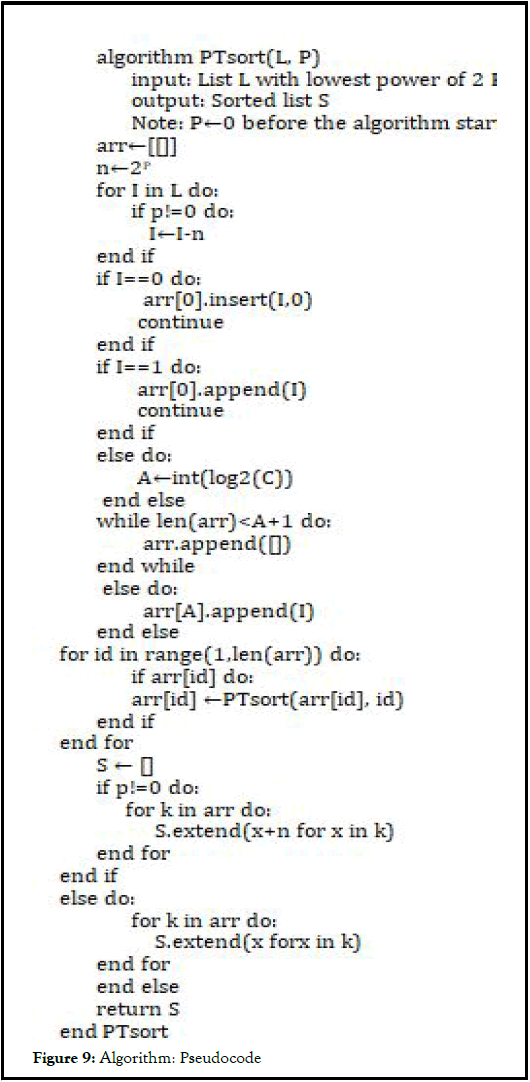
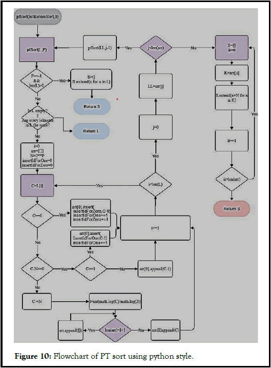
The following section displays the pseudocode and the flowchart of PT sort in Python style (Figure 2).
Example:
An example list is being sorted by PT sort in this section. Using random number generator, we get a list L with 10 numbers which is the value of n.
Steps:
• Create a new empty list arrx which recursion layer, x, is 0. The largest power of 2 number, P, is 0 in the first layer (Figure 3).
• Loop the list L. For every element C, the first element of the list is 45.
• log2 C is being calculated and taken the integer part. In this step, log2 45 have the value 5.
• Check if the arrx has ⌊ log2 C ⌋ sublists where ⌊⌋ is the floor function, which gives the largest integer less than or equal to x. If it has, add C into the sublist with index 5. Otherwise create the sublists and add C into it. If the layer x is not 0, the numbers should substract 2P before adding into the sublist (Figures 4 and 5).
After looping the whole L, the arr0 should be this:
• In the arr, each sublist contain numbers that the numbers are in the range of 2i<C<2i+1 where i is the index of the sublist. In Figure 6, 31 and 17 (before substract) are in the sublist with index 4.
• After processing all the elements in the L. PT sort uses recursion on each of the sublists. arr0 is going to be L and arr1 is created. If the sublist is empty, only has all same values, or only contains 0 and 1, the process of the current sublist is done. Otherwise, apply steps 1 and 2 to every sublist. Figure 6 is [31,17], with P=4, in arr0. After applying step 1 and 2, it becomes arr1 in Figure 6:
• From the instruct in Figure 7, all the sublists in the arr1 are done. Every element in the sublists form to a list S after add of the numbers that they are substrate, using C+2P. After adding back. The elements in sublists of arr1 are conbined and return. The (31,17) in arr0 is replaced by the new list (17,31) which is after processed.
• Then, PTsort is processing the next sublist in arr0 which is (45,37,34,35). Using the same stepts. A sorted sublist replaces the current sublist. This also apply on the next sublist.
• Combine all elements in sublists of arr0. They do not need to add numbers because arr0 does not substract numbers (Figure 8).
Analysis
The results show in Figures 9 and 10.
Flowchart: PT sort
Results and Discussion
In the first section of this part, PT sort compares to another sorting algorithm which appears in the Introduction. The following section shows the performance of PT sort. The performance of PT sort. Graph comparing is an effective way to compare algorithms. However, there are certain drawbacks associated with the use of it. The main disadvantage is that the result depending on the code and other factors. The graph of the sort algorithm is for reference only. The time and space complexity of PT sort is proposing.
Compare to other algorithms
Merge sort: Merge sort has a great representative of the divide and conquer algorithm which is also applied on PT sort. That is why we compare merge sort with PT sort through merge sort is the only comparison sort that appears in this paper. PT sort and Merge sort both use recursion to traverse the lists.
Pigeonhole sort: Pigeonhole sort and PT sort are both non comparison sort. Pigeonhole sort use support array so does PT sort. Pigeonhole sort does not change the same value’s order, which means it is a stable sort technique. PT sort is also stable. Both sorting algorithms go linear time complexity when only the size of the list change.
Bucket sort: Bucket sort and PT sort is similar but also different. Bucket sort use “buckets”, and PT sort has support arrays. However, the range of the buckets are the same, but the range of support arrays depending on its index. Bucket sort, same as PT sort and other sorts, goes linear time complexity when only the size of the list change.
Counting sort: The main similarity between counting sort and PT sort is when the largest value of the sort increase, time cost also increases. Counting sort is an integer sort, so does PT sort.
Radix sort: The word “radix” has a huge connection for PT sort. Nevertheless, the principle between radix sort and PT sort is quite different. When the range of the list increase, digits also rise. Radix Sort is efficient with a large value key because the time cost decreases when the digit increases when PT sort has the opposite effect.
Performance
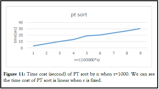
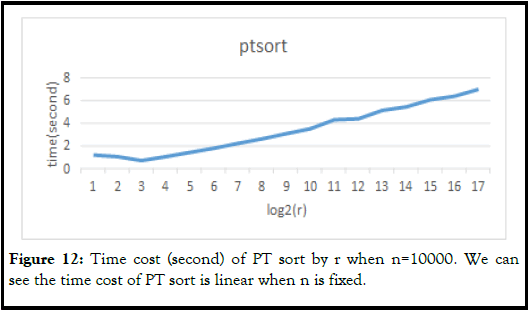
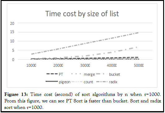
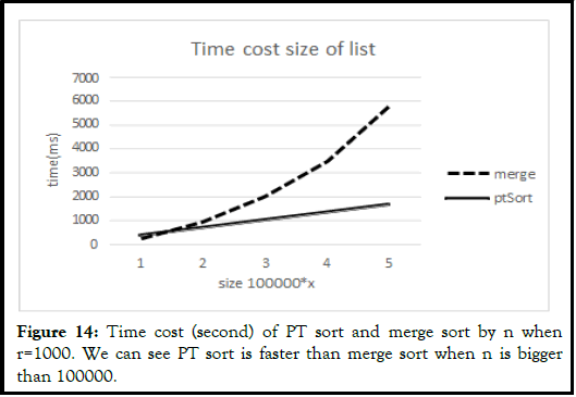
This section displays the line graph which shows PT sort and other sorts’ performance base on n, the list size, and r, the range of the list (Figure 11-14).
Time and space complexity
After comparing it to these famous sorting techniques; for example, bubble sort, selection sort, etc. The result shows that PT sort is more efficient than selection sort and bubble sort, and faster than merge sort when the range of list is under 1000 and size is bigger than 100000. The rate of change of time cost by the size of PT sort is much smaller than merge sort. The main disadvantage of PT sort is that the time cost increases significantly based on the range of numbers in the list.
The time complexity of PT sort is 0(n· log2 r)for best, average, and worst. The worst space complexity of PT sort is the same as time complexity which is 0(n. log2 r). PT sort is a stable sort because the order of the same value element does not change (Table 1).
| Algorithm | Average time complexity | Space complexity | Stable |
|---|---|---|---|
| PT | n â?? log2 r | n â?? log2 r | Yes |
| Merge | n â?? log2 n | n | Yes |
| Bucket | n + r | n + r | No |
| Pigeon | 2n + 2k | 2k | Yes |
| Count | n + r | n + r | Yes |
| MSD radix (in-place) | n â?? k | 2 | No |
Table 1: Simply compare the time complexity, space complexity and stability of these sorts.
Conclusion
In this paper, I have proposed a non-comparison sort, PT sort. PT sort is an integer sorting algorithm. Its average time complexity is 0(nâ?? log2 r), so does its space complexity. PT sort is stable. Its core idea is subtracting the element by the power of two. The experiment result shows that Pt sort is efficient when the range r is small. It can beat merge sort if the list size is big enough. There are two biggest disadvantages of PT sort. First, the time cost can increase significantly when r and n are both enormous. Second, PT sort cannot sort negative numbers. One way to fix it is to separate negative and positive numbers, using absolute value, and then reverse the list that contains negative numbers. The future of the PT algorithm is unknown, but it is worth to be explored.
References
- Thomas H, Cormen Charles E, Leiserson Ronald L, et al. Introduction to Algorithms. 2nd Edition. MIT Press and McGraw-Hill; United States; 2001.
- Donald E Knuth,. Section 5.2.4:Sorting by Merging. Sorting and Searching. The Art of Computer Programming. 2nd edition. Addison- Wesley; 1998.
- Merge sort. Wikipedia contributors; 2023.
- Black PE. "pigeonhole sort", in Dictionary of Algorithms and Data Structures, Paul E. Black, ed. 21 April 2022.
- Pigeonhole sort. Wikipedia contributors; 2022.
- Bucket sort. Wikipedia contributors; 2023.
- Edmonds Jeff. "5.2 Counting Sort (a Stable Sort)". How to Think about Algorithms. Cambridge University Press; United Kingdom; 2008.
- Sedgewick, Robert. "6.10 Key-Indexed Counting". Algorithms in Java, parts 1-4. Fundamentals, Data Structures, Sorting, and Searching. 3rd edition. Addison-Wesley; 2003.
- Radix sort. Wikipedia contributors. 2023.


