Solving a System of Linear Equations

Received: 23-Aug-2021 Accepted Date: Sep 07, 2021; Published: 14-Sep-2021

Citation: Obradovic D, Mishra LN, Mishra VN. Solving a system of linear equationss. J Pur Appl Math. 2021; 5(5):58:60.

This open-access article is distributed under the terms of the Creative Commons Attribution Non-Commercial License (CC BY-NC) (http://creativecommons.org/licenses/by-nc/4.0/), which permits reuse, distribution and reproduction of the article, provided that the original work is properly cited and the reuse is restricted to noncommercial purposes. For commercial reuse, contact reprints@pulsus.com

Abstract

The content of the system of linear equations makes it an interesting matter that can also be further expanded and deepened. The three methods most commonly used to solve systems of equations are substitution, elimination, and extended matrices. Replacement and elimination are simple methods that can efficiently solve most systems of two equations in a few direct steps. The extended matrix method requires several steps, but its application extends to a number of different systems. The elimination method is useful when the coefficient of one of the variables is equal (or its negative equivalent) in all equations.

Keywords

HIV; Stigma; Discrimination analysis; Northeastern Nigeria

Introduction

Solving a system of linear equations is one of the basic tasks of linear algebra. There are exact algorithms for solving systems, however when it comes to systems of larger dimensions (e.g. over 10,000 equations), most of these algorithms are not applicable in practice. One of the algorithms is Kramer’s rule or determinant method, but this algorithm is interesting only from a theoretical point of view. It is enough, for example, to prove that the determinant of the system is different from zero to know that the system has exactly one solution, ie in homogeneous systems that the determinant is equal to zero shows that the system also has nontrivial solutions. In practice, for a system of dimension n it is necessary to perform O (n!n) arithmetic operations, which speaks enough about the inadmissibility of this method for solving systems of large dimensions. A somewhat more acceptable method for solving the system of equations is the Gaussian elimination method (which will be implemented in this paper for comparison), the complexity of this method is O (n³).

Direct and Interactive Methods for Solving a System of Linear Equations

Methods for solving systems of linear equations are divided into direct and iterative. In direct methods, an exact solution is reached in a finite number of steps, while in iterative methods, the solution is the limit value of a series of consecutive approximations that are calculated by the method algorithm.[1] Two seemingly positive features of the direct method are the finite number of steps and the exact solution, however, as already mentioned, this finite number of steps is not feasible in real time, e.g. if Kramer’s rule solves a system of 10 equations with 10 unknowns, it will be necessary to perform about 10 • 10! Operation or over 36 million operations.

As for the accuracy of direct methods, it is absolute and retained only if there is no calculation error, which accumulates very quickly by division, which is a very common operation in direct methods, i.e. accuracy is retained if decimal numbers are not rounded to the final decimal number or a rational notation of a number runs through the whole method (unless irrational numbers are used) [2].

If we give up absolute precision (which in practice does not even exist because many bits are finally used to write real numbers), iterative methods can be much more useful, because large systems can be solved in real time - of the order of several tens of thousands, which is discretized. Different systems of linear equations just get different problems [3].

System of Linear Equations

The solution of a system of n linear equations with n unknowns is n numerical values, such that when they are replaced in the equations of the system, all n equations are satisfied.

A system can have a single solution, an infinite number of solutions and no solution (in the other two cases the systems are singular). There are two types of numerical techniques for solving systems of linear equations:

Direct methods - in the final number of steps we come to the correct solution,.

Iterative methods - we get an approximate solution with a certain accuracy [4].

From the direct methods we have: Gaussian method of elimination and its variants: with the selection of the main element and with the scaled selection of the main element.

In computational mathematics, an iterative method is a mathematical procedure that uses an initial value to generate a series of improvements of approximate solutions for a class of problems, in which the n-th approximation is derived from the previous ones. The specific application of the iterative method, including the termination criteria, is the iterative method algorithm. An iterative method is called convergent if the corresponding string converges for the given initial approximations. Mathematically rigorous analysis of the convergence of the iterative method is usually performed; however, iterative methods based on heuristics are also common.

In contrast, direct methods try to solve the problem with a final series of operations. In the absence of rounding errors, direct methods would provide an accurate solution (such as solving a linear system of equations. However, iterative methods are often useful even for linear problems involving many variables (sometimes of the order of millions), where direct methods would be overly expensive. in some cases impossible) even with the best available computing power.

By direct method we mean methods that theoretically give the correct solution a system in a finite number of steps such as Gaussian elimination. In practice, of course the resulting solution will be contaminated with a rounding error associated with the arithmetic is used.

Factorization Methods

We solve a system of n linear equations with n unknowns: . One of the approaches to solving the system is based on the LR-factorization of the matrix of system A, ie. reduction of A to the product: [5]

A=LR

where L is the lower-triangular matrix and R is the upper-triangular matrix. This is the system reduces to two triangular systems:

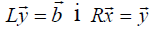
which are simply solved by successive substitutions. (Helecki Method)

In order for the LR-factorization to be unique, it is necessary to fix the diagonal elements of the matrix R or the matrix L in advance. Usually, a unit is taken for these values.

Factorization methods for solving of system of linear equations are based on factorization of matrix of system to product of two matrices in such form that enables reduction of system to two systems of equations which can be simple successive solved. In this section we will show up at the methods based on LR matrix factorization.

Iterative Processes

An iterative procedure is more efficient if the set task is completed in the shortest possible time. The efficiency of an iterative method is defined by introducing an efficiency coefficient. Efficiency can be introduced in several ways, but in such a way that it is proportional to the order of convergence of the iterative method (algorithm execution speed until fulfillment of some criterion or given accuracy) and inversely proportional to the work done, say the number of calculations of functions or numerical iterative operation.

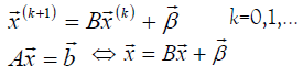
The simple iteration method can be described by the relation:

Sufficient string convergence condition towards the right solution is , wherein Arbitrary matrix norm:

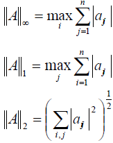(Schmidt’s norm)

A necessary and sufficient condition of convergence is that all eigenvalues of matrix B per module are less than one.

Jacobi’s Method

The implementation of Jacobi’s method has a lot in common with the implementation Givens methods. Here, too, instead of multiplying the starting matrix by the matrix rotations only calculate new values of those elements of the initial matrix which are modified. Stables are used to calculate the rotation matrix coefficients formula. The process of annulling the non-diagonal elements of a given matrix continues in the loop until the ratio of the non-diagonal norms of the current and the starting matrix becomes less than the desired accuracy ([6,7]).

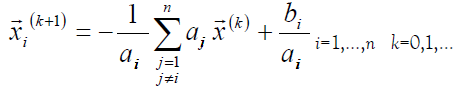
Jacobi’s method is a special case of the simple iteration method that is most often used:

That is, the components of the vector are determined by the formulas:

Convergence Conditions

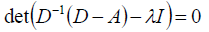– the roots of the equation should be less than one per module.

examine whether the matrix norm is less than one

If the conditions of the theorem on the dominance of the main diagonal of the matrix are satisfied:

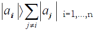
then Jacobi’s method applied to a given system converges independently of the choice of the initial approximation.

Many mathematicians have dealt with the problem of solving nonlinear equations and by finding the best and most efficient methods for calculating the mentioned problem ([8,9,10]). Everyone’s goal the improvement method was to start with Newton’s method and its modifications, with what fewer functional evaluations, the lower the degree of derivation, and the higher the order of convergence, comes to an effective method.

Gauss-Seidel Method

The Gauss-Seidel method is used to numerically solve a system of linear equations. This procedure speeds up the convergence process because it uses already obtained data from the previous iteration within one cycle. The convergence conditions are the same as for the Jacobi method [11].

The Gauss-Seidel method is a modification of the simple iteration method which achieves the acceleration of convergence. The system is given:

Where in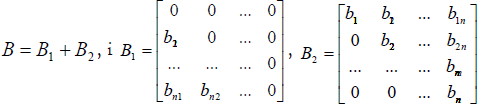

We form an iterative process of shapes:

The condition of convergence is: That all the roots of the equation 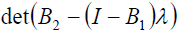be modulo less than 1; or that the main diagonal dominance theorem holds: 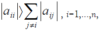in which case the given system converges regardless of .

As the Gauss-Seidel method to solve linear systems usually produces better results than the Jacobi method, we can expect a similar behavior for the Gauss-Seidelization process in the nonlinear case. Eventually, this could be used to increase the speed of convergence of the original iterative method [12].

Iterative Methods for Matrix Inversion

Let it be 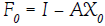a matrix representing a measure of the deviation of the matrix , approximation A^-1 from A^-1.

Let’s define through matrices:

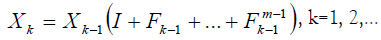
If it is , through the matrix {X_k} converges to A^-1.

Schultz Method for Matrix Inversion: 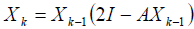(za m=2, what is most used in practice is the Schultz method)

The efficiency of the method is demonstrated with the help of matrices arising in the numerical solution of a hypersingular integral equation (namely, the Prandtl equation) on a square.

The iterative method will be extended by theoretical analysis to find pseudo-inverse (also known as Moore-Penrose-inverse) singular or rectangular matrix [13].

Determining the Eigenvalues of Matrices

The scaling method is used to determine the dominant eigenvalue λ₁ value. Vector represents in each step an approximation for an un-normalized eigenvector corresponding to the eigenvalue λ₁. However, in practice, instead of a series of vectors uses string defined by formulas:

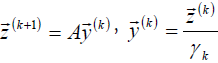, wherein:

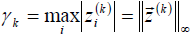, i tada je

For the initial vector we take some approximation of our own vector , if such an assessment is known to us in advance. If this is not the case it is taken .

Conclusion

Systems of equations can be solved using several methods: substitution, opposite coefficients, graphical, determinants, etc. All methods lead to the same solution, and which of them will be used depends on the task setting (you should choose the method that seems most suitable for solving in the given task).

Direct methods try to solve the problem with a final series of operations. In the absence of rounding errors, direct methods would provide an accurate solution (such as solving a linear system of equations.

Iterative methods are often useful even for linear problems involving many variables (sometimes of the order of millions), where direct methods would be overly expensive. in some cases impossible) even with the best available computing power.

Factorization methods for solving of system of linear equations are based on factorization of matrix of system to product of two matrices in such form that enables reduction of system to two systems of equations which can be simple successive solved. In this section we will show up at the methods based on LR matrix factorization.

The implementation of Jacobi’s method has a lot in common with the implementation Givens methods. Here, too, instead of multiplying the starting matrix by the matrix rotations only calculate new values of those elements of the initial matrix which are modified. Stables are used to calculate the rotation matrix coefficients formula.

The Gauss-Seidel method is used to numerically solve a system of linear equations. This procedure speeds up the convergence process because it uses already obtained data from the previous iteration within one cycle. The convergence conditions are the same as for the Jacobi method.

Systems of equations in which there is only one solution (i.e. one ordered pair of solutions) are called certain systems. Apart from them, there are also indeterminate systems (systems that have infinitely many solutions) and contradictory (impossible) systems (systems that have no solutions).

REFERENCES

1. Noreen J. A comparison of direct and indirect solvers for linear system of equations. Int J Emerg Sci 2012; 2:310-21.
2. Duff IS, Erisman AM, Reid JK. Direct methods for sparse matrices. Oxford University Press, UK; 2017.
3. Axelsson O. Solution of linear systems of equations: iterative methods. In Sparse matrix techniques 1977. Springer, Berlin, Heidelberg: 1-51.
4. Young DM. Iterative solution of large linear systems. Elsevier; 2014.
5. Okunev P, Johnson CR. Necessary and sufficient conditions for existence of the LU factorization of an arbitrary matrix. arXiv preprint math/0506382. 2005.
6. Sleijpen GL, Van der Vorst HA. A Jacobi--Davidson iteration method for linear eigenvalue problems. SIAM review. 2000; 42:267-93.
7. A Jacobi–Davidson iteration method for linear eigenvalue problems SIAM J Matrix Anal Appl 17. 1996; 401-425.
8. Crowder H, Wolfe P. Linear convergence of the conjugate gradient method. IBM J Res Dev 1972; 16:431-3.
9. Wolfe P. Convergence conditions for ascent methods. SIAM Rev. 1969; 11:226-35.
10. Lenard ML. Practical convergence conditions for unconstrained optimization. Mathematical Programming. 1973; 4:309-23.
11. Niki H, Harada K, Morimoto M, Sakakihara M. The survey of pre-conditioners used for accelerating the rate of convergence in the Gauss– Seidel method. J Comput Appl Math 2004; 164:587-600.
12. Li W. A note on the preconditioned Gauss–Seidel (GS) method for linear systems. J Comput Appl Math 2005; 182:81-90.
13. Guo CH, Lancaster P. Iterative solution of two matrix equations. Math Comput 1999; 68:1589-603.