The d’Alembertian operator and Maxwell’s equations

Received: 16-Nov-2018 Accepted Date: Nov 30, 2018; Published: 10-Dec-2018

Citation: Cassano CM. The d’Alembertian operator and Maxwell’s equations. J Mod Appl Phys. 2018;2: 26-28.

This open-access article is distributed under the terms of the Creative Commons Attribution Non-Commercial License (CC BY-NC) (http://creativecommons.org/licenses/by-nc/4.0/), which permits reuse, distribution and reproduction of the article, provided that the original work is properly cited and the reuse is restricted to noncommercial purposes. For commercial reuse, contact reprints@pulsus.com

Abstract

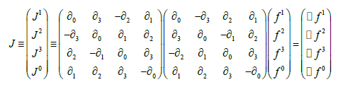
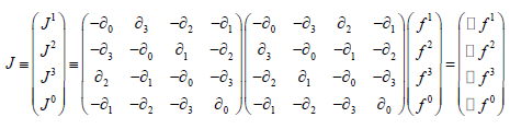
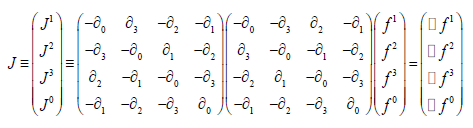
The d’Alembertian is a linear second order differential operator, typically in four independent variables. The time-independent version (in three independent (space) variables is called the Laplacian operator. When its action on a function or vector vanishes, the resulting equation is called the wave equation (or Laplace’s equation). When it’s action is identified with a non-zero function (or vector function) the resulting equation is called Poisson’s equation. This equation is fundamental to and of great importance in field theory. The focus of this tutorial is to demonstrate that when acting on a four-vector, the d’Alembertian may be factored into two 4 x 4 differential matrices. This d’Alembertian operator factorization of a four-vector into two 4 x 4 differential matrices is not merely another form of expressing Maxwell’s equations; but remarkably, yields a quantum and unified field theory generalization.

Keywords

Maxwell’s equations; Unified field theory; d’Alembertian; Differential operator; Mathematical physicssection; Isoperimetric theorem; Curvature

Introduction

The d’Alembertian is a linear second order differential operator, typically in four independent variables. The time-independent version (in three independent (space) variables is called the Laplacian operator. When it’s action on a function or vector vanishes, the resulting equation is called the wave equation (or Laplace’s equation). When it’s action is identified with a non-zero function (or vector function) the resulting equation is called Poisson’s equation. This equation is fundamental to and of great importance in field theory. The focus of this tutorial is to demonstrate that when acting on a four-vector, the d’Alembertian may be factored into two 4 × 4 differential matrices.

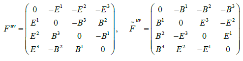
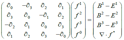
Many field theory books denote electromagnetic field tensor and dual tensor (including [1-3]), respectively, in 4 × 4 matrix form, as follows:

yielding Maxwell 's equation as :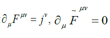

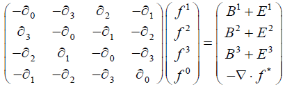
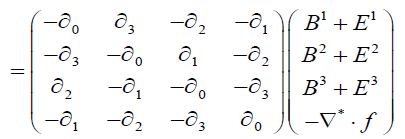
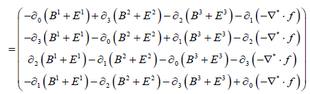
Noting the sum and difference of these matrices, then defining:(Using the same Einstein summation convention)

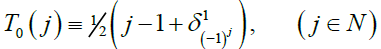
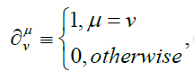(the Kroenecker delta function)

(1)

and:

(2)

B − E :

(3)

and:

(4)

B + E :

(5)

and:

(6)

Then,

and:

(remembering that )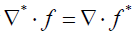

Subtracting:

These may be expressed as:

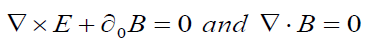(7)

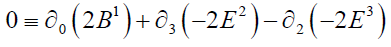
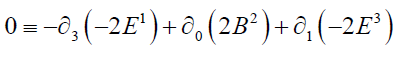
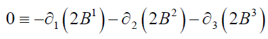
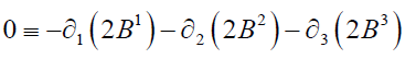
are the Homogeneous Maxwell’s Equations,

Satisfied identically, due to the definitions of E and B .

Adding:

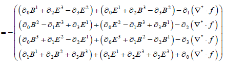
Continuing, from (6):

(7)

(8)

(9)

(10)

(11)

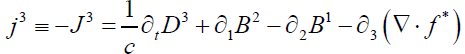
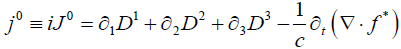
At this point, one may define:

x⁰ = ict, f ⁰ = iφ , D = iE

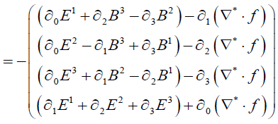
Then:

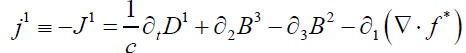
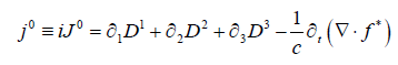(12)

(12)

These are the Inhomogeneous Maxwell’s Equations

Notable definitions for current/charge densities are (for the various, respective guages):

Representation I:

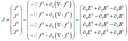(13)

Representation II:

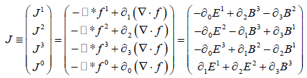(14)

Note: The field equations are invariant for all f such that:

In representation I:

(15)

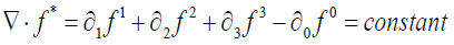
In representation II (Lorentz representation):

(16)

(This is commonly called the Lorentz Gauge)

Clearly, another representation comes to mind:

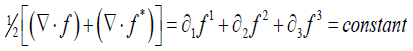(17)

(Commonly called the Coulomb or Radiation Gauge)

This d’Alembertian operator factorization of a four-vector into two 4 × 4 differential matrices is not merely another form of expressing Maxwell’s equations; but remarkably, yields a quantum and unified field theory generalization.

REFERENCES

1. Ryder LH. Quantum field theory. Cambridge University Press. Cambridge, UK. 1986.
2. Kovetz A. Electromagnetic theory. Oxford University Press, Inc, New York. 2000.
3. Graham W. The Cambridge handbook of physics formulas. Cambridge University Press, New York. 2000.