
Ulianov perfect liquid model explaining why matter repels antimatter
Received: 12-Nov-2023, Manuscript No. puljpam-23-6851; Editor assigned: 15-Nov-2023, Pre QC No. puljpam-23-6851 (PQ); Accepted Date: Jan 29, 2024; Reviewed: 18-Nov-2023 QC No. puljpam-23-6851 (Q); Revised: 21-Nov-2023, Manuscript No. puljpam-23-6851 (R); Published: 31-Jan-2024, DOI: 10.37532/2752-8081.24.8(1).01-14
Citation: Ulianov PY. Ulianov perfect liquid model explaining why matter repels antimatter. J Pure Appl Math. 2024; 8(1):01-14.
This open-access article is distributed under the terms of the Creative Commons Attribution Non-Commercial License (CC BY-NC) (http://creativecommons.org/licenses/by-nc/4.0/), which permits reuse, distribution and reproduction of the article, provided that the original work is properly cited and the reuse is restricted to noncommercial purposes. For commercial reuse, contact reprints@pulsus.com
Abstract
This paper presents a new model for generating mass of materials particles that is compatible with the theory of general relativity and some aspects of quantum mechanics. The new model was called Ulianov Perfect Liquid or UPL model.
The UPL model arises from a very simple idea, which is to observe the foundations of the models of perfect liquid (ie a liquid without friction and without viscosity) that are used to model problems in the framework of general relativity.
If indeed the space time continuum can be simulated using models of perfect, why we can’t assume that there is in fact some kind of perfect fluid, from which spacetime emerges?
Considering this possibility, the authors did a real breakdown of a perfect liquid, linking it to "space-time atoms” that behave as ideal spheres, which were named Ulianov Spheres or uspheres.
The UPL model allows us to observe the emergence of matter and antimatter, derive the law of gravitation and some equation obtained from general relativity (Schwarzschild equation) and also explains the origin of inertial mass.
Moreover the UPL model shows us some repulsive forces arising from the iteration between particles of matter and antimatter, what is presented in this paper.
Key Words
Liquid model; Antimatter; Viscosity
Introduction
Until the early twentieth century it was believed that light traveled through space in a kind of ether, which led physicists to develop a series of experiments such as the Michelson Interferometer, whose objective was to measure the speed Earth in relation to the Ether [1]. The results showed an intriguing finding: The light always traveled at a constant speed regardless of the speed of the Earth. These results were one of the starting points for Albert Einstein formulated the theory of special relativity presented in 1905, which overthrew Newtonian paradigm of absolute space and absolute time and abolished the concept of Ether. However, many theoretical and experimental work has shown situations in which the ether is still considered [2].
An important experiment was conducted physical R. D. Witte who in 1991 worked with the synchronization of atomic clocks. Witte got results that pointed to some sort of ether that would reference the Earth speed in space [3].
Witte failed to publish their experimental results, why they apparently contradicted the principles of Einstein's relativity. On this way the data obtained by Witte was only recognized as true in 2006 when R. T. Cahill showed that they were compatible with the principles of special relativity [4].
Same as the concept of Ether lost its entire acceptance in modern physics models, both the experimental work of Witte as the theoretical explanations of Cahill were virtually ignored by the scientific community until today.
Currently some of the theories such as the quantum gravity has used the most modern concept of ether, defining "space atoms" to describe space-time distances in order of the Planck length (10-35m) [5,6].
These new model of ether arise also in the theory of general relativity, where the Einstein´s field equations are difficult to solve and require some “tricks” to simulate more complex problems. Ono of this tricks are the use of simulators that consider the behavior of an perfect liquid, a liquid without friction and without viscosity, that have physical behavior equations that resemble those defined in general relativity.
Based on this scenario the authors believe that space-time can indeed be described as a kind of perfect liquid, called Freeman Ulianov Perfect Liquid (UFPL), which is basically composed of a network of finite spatial atoms, and these atoms have some parameters, associated with pressure and if energy density.
A UPL is not static and expands the time axis, growing continuously. Thus each atom space-time in the model UPL, was associated with a perfect sphere, that subject to internal and external pressures and brings a certain energy density. The model defines these UPL perfect spheres with the name Ulianov Spheres or usphres. Each usphere has its diameter equal to the Planck length.
As two uspheres by touching a single infinitesimal point, the friction force between them is zero, and together they act as a perfect liquid network.
The UPL model is able to describe some important properties of matter and antimatter and points to a condition in which the particles of matter tend to repel the particles of antimatter. Furthermore the model UPL matter particles distort network usphere generating negative pressures that collapse some of the spheres, generating uspheres of zero radius which were named Ulianov Holes or uholes. A uhole behaves as an elastic hole having two extremities, one extremity (named uhole) associated with matter and another extremity (named antiuhole), which is associated with antimatter.
When an uhole finds an antiuhole they are annihilate each other. In terms of pressure and thus annihilation suggest a model where one antiuhole generates positive pressure (associated to one particle of matter) and one uholes generates negative pressure (associated to one particle of matter).
In UPL model the mass of one particle is connected to the pressure value in the uhole associated to this particle, which in turn generates the concept of negative mass, set within a new context, which will be discussed below.
Negative Mass
In 2011 the Italian physicist, Mario Villalta proposed that the gravitational force between particles of Matter (M) and Antimatter (AM) tends to be repulsive, as shown in Figure 1 [7].

Figure 1: Forces acting on different types of matter.
Figure 2 shows the forces that arise between each kind of electric charge of which forces can be calculated by Coulomb's law:


Figure 2: Forces that act on different types of electric charge.
Considering the forces shown in Figures 1 and 2, an analogy can be observed between the behavior of electric charges and a massive particle.
In 1928 the British physicist Paul Dirac modeled the positron theory, predicting the existence of antimatter. In Dirac original ideas the positron mass should be considered negative.
Unfortunately a comprehensive application of Newton's first law leads physicists to consider that a body with negative mass accelerates in the opposite direction of the applied force, something that contradicts a series of basic postulates of physics, creating the idea that the mass cannot be negative.
On the other hand, when Newton formulated they first law, certainly not was considered the existence of antimatter.
On this way, the authors are proposing that Newton's first law should be modified to:

In the context of equation (2) a body may assume a mass negative value, and thus accelerate even in the same sense that a resulting force is applied to it.
Likewise considering that the Villalta model is correct; if we assume that the mass of antimatter is negative Newton's law of gravitation can be redefined as:

Since the negative sign arises to maintain the same reference to the electrical charges case, where equals charges repel itself, while between equal types of masses appear attractive forces.
The use of a negative mass also requires adjustments in the formula that calculates the kinetic energy contained in particles of matter and antimatter:
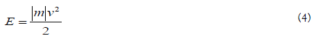
The module function can be used in all formulas that apply the mass as one parameter, whenever it is applied to a context that considers the existence of antimatter particles where the mass can be considered as negative [8-15].
The authors believe that the use of the module function avoids all the problems that arise from using a antimatter negative mass and moreover provides a number of benefits, such as the law of gravitation defined in equation (3) that allows describe all interactions between matter and antimatter that was shown in Figure 1.
Mass Annihilation
Considering that the mass of antimatter is negative Einstein formula that relates matter and energy must also be modified to include the function module:

The conversion of matter into energy defined by equation (5) will be complete when a matter particle finds a particle of antimatter. In this case the particles masses annihilate leaving only energy. In this context a negative value for an antimatter particle mass can naturally annihilate the positive mass of a matter particle because de sum of its masses is equal to zero [16-19].
Figure 3 shows an example where a proton and an antiproton colliding and annihilating itself generating energy. Whereas the proton mass Mp is equal to antiproton mass, if we assume that the antiproton mass is negative (-Mp), the total mass (Mtotal) in Figure 3 will be zero (in all frames) and when the particles lie at the same point they mass will cancel will cancel one another, generating energy.

Figure 3: Annihilation of an electron with a positron generating energy.
Figure 4 present the same case of Figure 3, with another proton added. If the law of gravitation be applied, we can observe tow gravitational forces arising in proton 2 as shown in frame (a) on Figure 4.

Figure 4: Forces which arise between particles before and after the annihilation.
After the annihilation process, the two forces represented in frame (b) in Figure 4 will be equal to zero, because will not have more mass to iterate with proton 2.
However for the frame (a) there are two possibilities:
• In the traditional model where matter and antimatterattract itself, the forces F1 and F2 have the same directionand intensity. In this case the proton 2 is attracted, untilthe time when the particles are annihilating, and so theforce goes to zero.
• In the model proposed by Villalta, the force F2 has theopposite direction of the force F1 generating acancellation. Thus there will be no discontinuity in theforce acting in proton 2, due to annihilation of theparticles.
General relativity broke paradigm of Newtonian gravitational force acting at a distance defining a new paradigm where the presence of matter distorts space time. So for example, the orbits of the planets in the solar system can be explained when the sun matter distorts space time forming geodetic trajectories, as shown in Figure 5.

Figure 5: Espaço distorcido formando trajetórias geodésicas.
Figure 6 shows a classic example of two dimensional space, defined by a network of parallel lines, where the presence of mass at a central point "shrinks" the space.

Figure 6: Dimensional space being distorted by the presence of matter.
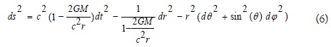
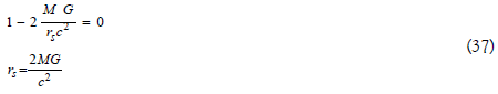
In general relativity the distortion generated by a spherical body with mass M, can be calculated, using the field equations defined by Einstein, generating the Schwarzschild equation:
Looking at the Figure 4 example in the context of General Relativity, will also has two analysis options:
In the traditional model where matter and antimatter have positive mass, the distortion caused by the proton mass is the same caused by the antiproton mass. This can be easily seen from equation (6) which does not differentiate the proton mass and antiproton mass. On this way in Figure 4(a) we have a maximum distortion, that will be null at Figure 4(b). Here we have again a discontinuity generated by the mass annihilation process.
In the model proposed by the authors, antimatter has negative mass and so the distortion it causes in space tends to nullify the distortion caused by matter. Thus in Figure 4(a) the distortion generated by the proton mass is partially offset by the distortion generated by the antiproton mass, generating a continue transition until the total distortion is null when the tow particles is at the same position.
Considering that antimatter has a negative mass (-M) the equation (6) for space time distortion can be written as:
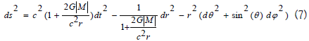
Equation (7) also defines the distortion caused by an antimatter black hole.
UPL Model
Within the general relativity, the field equations can be associated with a perfect liquid, ie an incompressible liquid, which has no friction or viscosity and can be completely described by its isotropic pressure and energy density.
A perfect liquid can be associated with an energy-momentum tensor (Tμv) which is analogous to the energy-momentum tensor used in general relativity field equation.
Simulations models based in perfect liquids allow for example to study the behavior of matter into stars, taking into account the effects of general relativity.
The authors believe that the perfect liquids models are more than mathematics "tricks", and so the real nature of spacetime can be associated with a type of perfect fluid, that are relating to some kind of "space time atoms".
In this context the authors propose a new model named Freeman Ulianov Perfect Liquid (FUPF) which goes beyond the traditional models of liquids perfect, considering a liquid formed by small spheroids, whose diameter is equal to Planck length. These small spheroids were named Ulianov Spheres (Uspheres) and behave with perfect spheres of the same radius that are associate forming a network, as shown in Figure 7. Where an usphere touch the adjacent usphere at only one point, will not be friction between them. On this way a tridimensional network of uspheres behaving as an incompressible perfect liquid.

Figure 7: Network uspheres forming a perfect liquid.
As the uspheres slide frictionless over one another the usphere network not have viscosity, the UPL is only characterized by the pressure and kinetic energy of each usphere that compose it.
In terms of pressure each usphere can be separately modeled as if it were a glass bubble placed a pressurized room, where there will be two pressures of interest, the inner pressure (inside the bubble) and external pressure (room pressure) (Figure 7).
Each usphere is modeled to maintain the same radius regardless of the pressures that is being submitted, except in the case where the internal pressure drops to zero, causing a usphere collapse where its radius becomes zero, composing a point particle that was named Ulianov Hole (uhole).
In the model UPL an empty volume of space can be associated with a uniform usphere network where the internal pressure is equal to external pressure, assuming a value (P0) which is constant throughout the liquid. The inclusion of a particle unit of this liquid matter is equivalent to applying a radial force field on a single usphere that transforms into an uhole.
Figure 8 shows a curve whit the values of inner pressure at a UPL on a point on which was inserted one uhole. In this curve, it can be seen that the pressure in the neighboring uspheres is also decrease. It is important to note that the influence of one uhole extends throughout the all UPL, generating a pressure variation that falls inversely with distance to the uhole position.

Figure 8: Internal pressure along an axis x which has been inserted uhole.
In the UPL model, we can also consider the value of pressure variation in each usphere defined by:

Thus the pressure in a uniform usphere network is defined as equal to zero and the creation of one uhole in this network, generates a negative pressure, as shown in the Figure 9 pressure curve.

Figure 9: UPL pressure along an axis x where has been inserted one uhole.
The UPL model associates an uhole to a matter particle, whose has positive mass. Furthermore UPL the model considers the existence of an antiparticle (of the uhole) called antiuhole, whose has negative mass and is associated with this antimatter (Figure 9).
The pressure generated by the presence of a antiuhole in a uniform usphere network is positive as shown in Figure 10.

Figure 10: UPL pressure along an axis x where has been inserted one antiuhole.
The curves shown in Figures 9 and 10 are equals but with opposite signs. Thus if we overlap one uhole and one antiuhole it´s generates a cancellation of the pressure curves, and so the usphere network becomes uniform again.
Gravitational Forces On The UPL Model
To analyze the forces that arise from the interaction of uholes and antiuholes we can use the analogy of a aquarium containing water on the earth surface. In this analogy one can consider the zero pressure ate de water surface. Deep in de water this pressure grows until a maximum value of pressure at the aquarium bottom. Looking again to Figure 8, we can associate the point where the UPL pressure is minimum (which is located near to the uholes) to the surface of the aquarium. On this way, the point where UPL pressure is greatest (far away from uholes) can be associated with the bottom of the aquarium. This leads to the scheme shown in Figure 11 where the surface of the aquarium is associated with high mass concentration (for example the earth's surface), whereas the pressure at the bottom of the aquarium is associated with a point in space, where the distortion caused by the mass becomes negligible.

Figure 11: Analogy of water pressure in a tank with the pressure UPL near to a body with mass.
Continuing the analogy we will be position two spherical bodies, inside the aquarium, one with higher density than water and the other with lower density, as shown in Figure 12. In this condition the body of greater density tends to fall, while the less dense body floats up to the surface.

Figure 12: Forces acting on two bodies placed in the aquarium.
Whereas in this analogy the water represents the UPL, the body with lower density can be associated with a uhole, a particle of matter with positive mass, which tends to move to the point of lowest pressure, going towards the planet surface. Thus in the UPL model a massive body loose on Earth, tends to fall toward the Eart surface, because the pressure in UPL is smaller (or more negative).
Likewise the body of higher density may be associated with an antiuhole, a antimatter particle with negative mass is, that tends to move the points with higher pressure, or in other words tends towards the outer space, moving away from the Earth.
It is important to note that in a antimatter planet, the UPL pressure would be greater in the planet surface, and so the lower density particle (matter) tends to move towards outer space, where the pressure is low. Whereas the higher density particle (antimatter) trend to move to the planet surface.
Another way to observe the particles iteration is shown in Figure 13. The iteration between two pressure curves generated by particles tends to attracted identical particles and repel particles whit opposing curves. This behavior can be best understood on the analogy of Figure 14, where a rubber line is placed between two walls of a aquarium, with a body attached to the rubber by means of a pulley.

Figure 13: Iteration of pressure curves generated by two distinct particles.

Figure 14: Two typical cases a body connected to an elastic line.
If the density of the body is greater than water it descends, the elastic stretching downwards. In case the density of the body being less than the water it rises up and the elastic also stretching.
In this analogy, if two bodies with same density are placed in the rubber line a little distance from one another, they tend to move to a same point as shown in Figure 15, where the arrows indicate the movement of each body

Figure 15: Two bodies whit same density connected to a elastic line.
Likewise if two bodies of different densities are placed on a same point of the elastic line, they tend to pull away as shown in Figure 16.

Figure 16: Two bodies with different density connected to a elastic line.
It should be noted that analogies presented in Figures 14, 15 and 16 only serve to better explain the interactions between massive particles. Figure 13 shows that the same type distortions tend to a same point generating a minimal end distortion. On this way opposing distortions tend to move away continuously.
Furthermore it is important to note that Figure 13 present basically the same forces diagram that was shown in Figure 1, where the matter attracts matter and repels antimatter, and vice versa.
Calculations of Pressures And Forces On The UPL Model
Assuming a uniform UPL where N1 uholes are inserted, they can be associated to a mass M1 is given by:

Since Kmu is the value of unitary mass, equivalent to a single uhole mass.
The UPL pressure at a distance d from the point where the mass M1 is positioned can be calculated by:
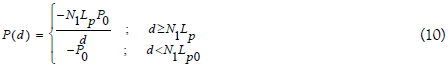
Where Lp is the Planck length.
Whereas a second set of N2 uholes is associated with a mass M2 which is given by:

The two sets of uholes (N1 and N2) are positioned at a distance d1, as shown in Figure 17, which also shows the pressure curve caused by the N1 uholes. For the second set of uholes we can consider the volume V2, associated with the N2 uspheres before its being compacted. In this case the N2 uholes isn´t formed and no generating variations of pressure on the surrounding uspheres.

Figure 17: Two sets of uholes positioned in a graph with a UPL pressure curve, caused by the group of N1 uholes.
Figure 17 presents an analogous behavior to a ball inserted in a liquid, which undergoes toward the surface. Considering that this ball has a volume V2 and a null density, it´s tends to move to regions of lower pressure in the UPL.
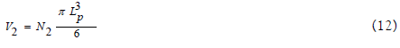
The value of V2 is equal to the volume of N2 usphere, each one with a diameter equal to the Plank length, that can be calculated by:
Under these conditions the force F, shown in Figure 16, can be calculated by:
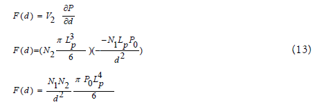
Applying equations (9) and (11) into equation (13):
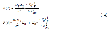
In equation (14) the constant K0 has its value expressed in m3 kg-1s-2, ie the same unit of Newton's gravitational constant (G). Thus whereas K0 equals G, equation (14) becomes the Newton law of gravitation.
Figure 18 shows an example of application of the new UPL model, where N uholes are positioned on a uniform usphere network. A force F is applied to these uholes, that passing to move with a speed v, which can vary in time.

Figure 18: Sets uholes being moved in a UPL.In (a) N uholes is moving and UPL is stopped; In (b) the volume V associated with the uholes is stopped and the UPL is moving.
In the frame (b) in Figure 18, we change the reference admitting that the uholes are stopped an the UPL moves at the speed v(t) (considered in the opposite direction).
Moreover in frame (b) the uholes are replaced by the volume associated uspheres before they are collapsed.
The moving UPL pressure can be calculated from Bernoulli's equation which describes the pressure behavior on ideal liquids:
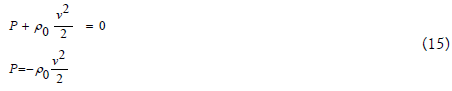
Where ρ0 is the UPL density.
Whereas an uhole has a mass equal to Kmu, calculating the volume of one usphere, the ρ0 value can be calculated as follows:
Under these conditions the force F, shown in Figure 18 can be calculated by:

Since the volume V is defined by N uspheres, its value is calculated by:

The pressure change with distance can be calculated based on equation (15):
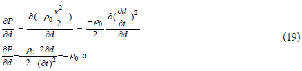
Where the parameter a is the fluid acceleration, ie an acceleration pointing in the opposite direction to the applied force. To use an acceleration reference in the same direction of the applied force, equation (19) should be modified to:

Applying the equations (16), (18) and (20) into equation (17) yields:
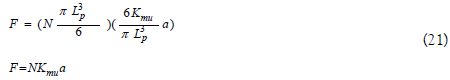
Whereas the mass M associated with N uholes is given by:

Thus using the equation (22) into equation (21) will be obtained first Newton's law:

Thus, the UPL model allows observing why the inertial mass assumes the same value as the gravitational mass. In both conditions the mass may be associated with a volume of spheres to be compacted into a perfect liquid, and this volume will be subjected to pressure variations, which may arise due to proximity to other bodies and also arise by the movement of the volume considered in the perfect liquid.
The UPL model also allows explain the planetary orbits without resorting to gravitational or centrifugal forces. In Figure 18 a body M1 is being orbited by a smallest body M2 that travels at a speed v in a circular orbit having a radius equal to d1.
In Figure 19 the body M1 generates a pressure drop which varies with the distance and generating regions of constant pressure over spherical shells centered in M1. Thus the dotted circle in this figure represents the orbit of M2, where the pressure will be constant, and can be calculated by:
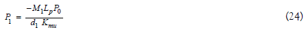

Figure 19: Body with mass M2 orbiting body with mass M1.
Besides the fact M2 body is moving at a constant speed, generating thereon a condition that negative pressure is given by:
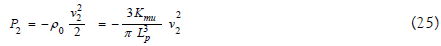
Thus M2 body tends to move in a trajectory in which the pressure P2 equal to pressure P1, as shown in the graph of Figure 20.

Figure 20: Pressures along a line drawn from the body M1.
To calculate the relationship between distance and orbital speed we can equate the equations (24) and (25):
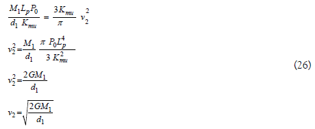
The body M2 does not suffer the effect of any force, and therefore it moves following lines with the same level of pressure, forming a circular orbit around the body M1.
Multiple Representations of The UPL Model
The UPL model can be interpreted by some observers in different ways. Each observer can see an entirely different universe, depends on this point of view.
This occurs because the set of models that describe the UPL is the result of a particular "filter" which is applied by the observer to "sees” certain aspect of UPL.
In deductions presented in the previous section, this feature was used without being explicitly mentioned. This occurred at the time that modeled a uhole, which is a particle having a mass and can be observed in two different ways.
To better understand this aspect it should be noted the process of forming a uhole starting from a UPL uniform, as shown in Figure 21.

Figure 21: Formation of a uhole in a uniform network and associated pressures.
As part (a) of this figure can be observed one UPL composed only usphres, and six uspheres were highlighted in yellow in order to generate a reference position. In this case the internal pressure of all uspheres is constant and equal to a value P0. As part (b) one usphere was painted black indicating that it is being "emptied" with its internal pressure being equal to zero, as indicated in the graph. As part (c) generating a usphere is collapsed uhole which ceases to exist in the network, as indicated by a black dot in this case the neighboring uspheres change position in order to take up the space freed in creating and moreover the uhole uspheres neighboring decreases in pressure as shown in the graph.
The uholes can then be observed under two distinct aspects:
• Particle punctual - in this case the uhole have the formshown in Figure 21-c, making a point particle with zerovolume and that affects the whole UPL generating apressure gradient that spreads through neighboringuspheres;
• Usphere with zero pressure - the uhole this case have theform shown in Figure 21-b, with a volume equal tousphere but with internal pressure equal to zero. In thiscase the uhole uspheres not affect neighbors.
Figure 22 illustrates the process of forming a antiuhole, which also can be considered two representations. Within the framework 22-bo antiuhole only bending pressure without affecting the pressure in neighboring uspheres, while in co-antiuhole affect the pressure across the UPL in which it is inserted.

Figure 22: Formation of a antiuhole in a uniform network and associated pressures.
Although the representations shown in Figure 21-b and 22-b are unrealistic from the point of view that UPL is not affected, they are very useful to calculate how a uhole antiuhole or react to changes in pressure UPL.
In this case an analogy can be established similar to that shown in Figure 12 where in a water tank with two spheres are positioned, one with higher density than water (associated with antiuhole) and one with lower density than water (associated with uhole). From a uniform UPL, a pair uhole/antiuhole past may be formed of any pressure usphere to one another as shown in Figure 23. In the model UPL density can be directly associated with the pressure and thus the density of a uhole will be zero while the density of antiuhole be two times greater than the density of UPL. This means that if we consider that the mass of a mass associated usphere is equal to the mass of a KMU antiuhole 2 Kmu equals the mass of a uhole equals zero (Figure 23).

Figure 23: Formation of a pair uhole/antiuhole in a UPL.
It is also possible to use a relative representation, defining the dignity of UPL as being equal to zero, and thus the mass of a uhole equals-KMU while the mass of a antiuhole equals KMU. However in the model are associated UPL the uholes matter and antiuholes are associated with antimatter, and more convenient to consider the mass of a uhole is positive (KMU) and the mass of a antiuhole is negative (-KMU). In this model, considering one uhole negative pressure (-P0) and a antiuhole positive pressure (P0), the mass of a usphere can be defined by the following equation:

Model UPL Related To General Relativity
Besides the alternative ways for representing and uholes antiuholes above, the model also considers UPL two forms of representation of usphres:
• Uspheres constant radius - all uspheres this embodimenthas the same radius which is equal to half the distancePlanck. In this case basically are observed pressurevariations in uspheres. This representation considers theviewpoint of a point particle (a uhole) which traverses theUPL, "jumping" from one usphere. To this particleuspheres all have the same size and distance measurement is accomplished digitally by counting the uspheres;
• Uspheres with variable radius - this representation canincrease the uspheres radius and thus tend to maintain aconstant internal pressure. Figure 24 shows such a set ofuspheres which increased in size due to the presence ofthree uholes on one point (indicated in white in thefigure). In this representation the distances are measuredbased on real numbers, taking into account the size ofeach usphere.

Figure 24: Representation of uspheres with variable size.
These two types of representation uspheres can be seen together in Figure 25, where the table (a) uspheres are distorted by the presence of uholes and under (b) are uspheres uniform. In this figure we can see that the blue rectangle drawn under (a) becomes a trapeze indicated in red under (b), but this trapeze angles remain equal to 90 degrees, because despite the space (a) be flat its representation shown in (b) is not associated with a Euclidean space.

Figure 25: a) UPL uspehres with variable radius. b) UPL usperes with fixed radius.
It is important to note that the presence of a uhole UPL in a uniform tends to increase usperes territories that occupy the space left by the collapse of usphere that generated the uhole. In the case of a uniform UPL is inserted antiuhole where it will increase in size due to it being subjected to increased internal pressure.
The theory of general relativity had broke the paradigm of Newtonian absolute space and time and constant, introducing a new paradigm within which the presence of matter and energy distort space-time. Looking back at Figure 5, which shows a two-dimensional space distorted by the presence of matter, we can say that the matter "shrinks" the space. However UPL in the model, considering the depiction of uspheres variable radius, shown in Figure 22, we can state that in fact the presence of matter expands the space.
This aspect can best be seen in Figure 23 where it was considered the same two-dimensional space of Figure 5 and are shown two enlarged details (red circles) uspheres of forming this space inside the representation of variable radius. In this representation the lines forming the grid are parallel and are not distorted, but uspheres the center of the figure are much higher because there is a large number of uholes the central position. Likewise uholes the farthest from the center will be smaller because they are less affected.
In Figure 26 the presence of seizing area (uholes) increasing the size of uspheres that are closest distance observed between the parallel lines will decrease when the number is considered the "home" space separating one row from another, as can be seen in this Figure.

Figure 26: Dimensional space distorted by the presence of uholes, being observed on the standard variable-sized uspheres.
The analysis of the distortion caused by N uholes positioned on a same point in space (i.e. in the same usphere) can be performed simply with the help of Figure 27. As part (a) of this figure we see an example where N equals three and five thus observed that black balls aligned re3presentam uspheres to be collapsed due to the presence of three uholes. Figure 28 shows superimposed uholes occupy a greater volume than the volume of uspheres 3. This behavior can be observed based on the analysis of equation 10, where N nothing increment the minimum pressure value (-P0) covers a larger volume, which is proportional to N3. Thus for each N uholes allocated on the same point will be observed N3 uspheres being compacted.

Figure 27: Adding uholes to an network of uspheres. (a) Original network, (b) New network with uspheres fed; (c) New uspheres network with fixed radius.

Figure 28: Three uholes focusing on a single point in a network usphere dimensional; (a) Top view, (b) Cut side.
In Figure 27-b uspheres the five black collapsed forming a single uhole, it ceases to be seen as a physical being, but to increase the radius in neighboring uspheres it provokes. We can observe in the table (b) that the yellow balls that were distant are playing each other and that their size has increased considerably in order to occupy the space generated by the compression of uholes.
In Figure 27-ca distorted network is seen from the point of view of particles that jump from one to another usphere in one "jump" regardless of the size assumed by them.
Also in Figure 27a, one can observe axis r in which it was indicated that a distance r1 in this example is equal to 7 uspheres. Under (c) we can see that this new distance (obtained after compression) was called and is now worth only 4 in this example (Figure 28).
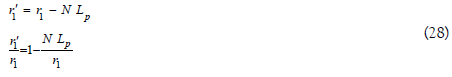
Since each usphere has a diameter equal to Planck length, a relationship between the distance and the distance r1 can be calculated as follows:
In Figure 27 networks usphere shown in Tables (a) and (c) appear at different times making it difficult to analyze.
Figure 28 solves this problem by showing an example of a rectangular room to be distorted by the presence of a large number of uholes (Figure 29).

Figure 29: Rectangular room being distorted by the presence of uspheres. (a) normal room, (b) distorted room.
Considering that the room can be quite long we can assume that the wall indicated by the red triangle will not be modified, keeping the length r1. The wall indicated by the blue triangle and decreasing compressed size, assuming a value, but the blue triangle do not notice it because it also shrinks in proportion along with any rule he possesses. Under (b) we observe that the side wall was crooked, but each triangle still sees this as a straight wall, in fact if the red triangle emit a beam of light along the wall the same will follow in a line parallel to this, bending as well. Besides the curved wall gets narrower near the blue triangle, but this does not realize it because his ruler has also shrunk proportionately. Thus we may say that:
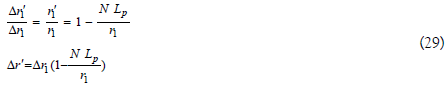
Applying equation (22) into equation (29):
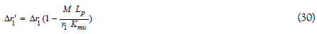
The value Kmu can be directly associated with the value of Planck mass which is given by:

being c the speed of light in vacuum and Planck constantcorrected.
The value of Lp is given by:

Applying (31) and (32) into equation (30):
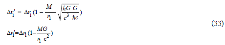
As the value Δr can be as small as desired it can be replaced by the derivative dr, which can equation (33) is generalized to:

As in the calculation of distances must be considered offset values squared equation (34) may be squared:
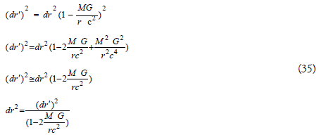
Equation 35 relates an infinitesimal displacement observed by the blue triangle; with the same displacement observe it at an infinite distance (point without distortion). Since the value that divides the displacement in equation (35) is positive and smaller than unity, the offset value will always be greater at infinity, so if for example the shorter side were multiplied by a factor of 0.8 red triangles could say that the width of the wall at infinity increased from 12.5 cm to 10 cm.
We can observe that equation (35) represents a part of the equation Schwarzschild, who is on the distortion of distances in three-dimensional space.
This shows that the model UPL can generate the same results as general relativity, but starting from a completely different basis.
Distortion in Space Caused by Antiuholes
Equation 35 relates an infinitesimal displacement observed by the blue triangle with the same displacement observe it at an infinite distance (point without distortion). Since the value that divides the displacement in equation (35) is positive and smaller than unity, the offset value will always be greater at infinity, so if for example the shorter side were multiplied by a factor of 0.8 red triangle could say that the width of the wall at infinity increased from 12.5 cm to 10 cm.
We can observe that equation (35) represents a part of the equation Schwarzschild, who is on the distortion of distances in three-dimensional space.
This shows that the model UPL can generate the same results that general relativity, but starting from one base totally distinta. É important to note that the reversal of antiuholes (antimatter) in a UPL generates a distortion similar to that shown in Figure 27. This occurs because the inclusion of N antiuholes in a single network point usphere generates a positive pressure that causes the usphese associated with antiuholes grow. As shown in Figure 29-b, "incorporating" uspheres some territories in order to have room to grow. Then the balls adjacent to antiuholes also expand causing the network shown in Figure 29-c. Considering the representation of uspheres with fixed radius shown in Figure 29-d can be seen that the presence of N antiuholes generates basically the same configuration of Figure 29-b due to the presence of N uholes.
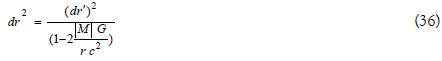
Thus the model UPL distortion generated by the presence of matter is practically equal to the distortion caused by the presence of antimatter, and equation (35) can also be deduced based on Figure 29, it is only necessary to consider the mass of the module, for the model UPL antimatter has negative mass:
Distortion in Space Caused by Antiuholes
Equation 35 relates an infinitesimal displacement observed by the blue triangle with the same displacement observe it at an infinite distance (point without distortion). Since the value that divides the displacement in equation (35) is positive and smaller than unity, the offset value will always be greater at infinity, so if for example the shorter side were multiplied by a factor of 0.8 red triangle could say that the width of the wall at infinity increased from 12.5 cm to 10 cm.
We can observe that equation (35) represents a part of the equation Schwarzschild, who is on the distortion of distances in three-dimensional space.
This shows that the model UPL can generate the same results that general relativity, but starting from one base totally distinta. É important to note that the reversal of antiuholes (antimatter) in a UPL generates a distortion similar to that shown in Figure 27. This occurs because the inclusion of N antiuholes in a single network point usphere generates a positive pressure that causes the usphese associated with antiuholes grow. As shown in Figure 29-b, "incorporating" uspheres some territories in order to have room to grow. Then the balls adjacent to antiuholes also expand causing the network shown in Figure 29-c. Considering the representation of uspheres with fixed radius shown in Figure 29-d can be seen that the presence of N antiuholes generates basically the same configuration of Figure 29-b due to the presence of N uholes.
Thus the model UPL distortion generated by the presence of matter is practically equal to the distortion caused by the presence of antimatter, and equation (35) can also be deduced based on Figure 29, it is only necessary to consider the mass of the module, for the model UPL antimatter has negative mass:
Black Holes with Schwarzschild Radius
The Schwarzschild radius defines the event horizon of a black hole, defined from the following equation:
Considering equations (29) and (33) we can establish the relationship:

Applying equation (38) in (37) will be obtained:

The value associated with this NLP length of the radius of the sphere of space that will be compressed when N uholes are positioned at the same point in the center of this sphere. Considering these uholes in compressed form this sphere of space, the turns into a dimensionless point. These form makes good sense that the event horizon of a black hole is associated with a shell sphere within which space and time are, compressed, and therefore cease to exist. What they want something from within this region of space actually is entering into a singularity.
However the event horizon of a black hole has twice the space tamenho ball being collapsed by the presence of N uholes. This factor two can be explained considering that in the position of a point in UPL there is uncertainty which normally Lp +-valley distance units. In Figure 30 is an example where 3 uholes are positioned in a uniform network, generated a sphere of radius equal to 3 Planck lengths. However by placing a dot in the center of this sphere will be an uncertainty, which is indicated by the blue arrows. This means that the axis of the coordinate system under consideration in measuring distances which may be in either center point of the circle is larger than the area to be compacted.

Figure 30: Adding N antiuholes in a network uspheres. (A) Original network; (b) growing Antiuhole incorporating neighboring usphres (c) Uhspreses neighboring increase in size, (d) Usphres observed with fixed radius.
The uncertainty of the source position of the shaft shown in Figure 30 can be seen Also the uncertainty about the position of the region of space that is compressed by N uholes. This is shown in Figure 31 That considers the two-dimensional space where the area to be compact by uholes is Indicated by red circles That can be defined in Several different positions. The blue circle shown in this figure Indicates the position of the event horizon Associated with black hole mass M, Which Is equivalent to N uholes. These form the equation 36 Relates directly to the event horizon That region of space will be compact by uholes Which Within the space-time itself ceases Becoming a singularity.

Figure 31: Adding N uholes in a uniform network.
Equation (36) shows that a single uhole mass can be associated with a micro black hole event horizon equal to twice the Planck length. So a uhole is the smallest black hole that may exist and its mass is equal to the Planck mass.
Time in UPL Model
In the model UPL time is deemed to have digital nature. In figure 32 are defined a series of "time frames", each containing a copy of a network usphere. In this case point particles (uholes) moving in UPL, passing from one position to another, as shown in Figure 32.

Figure 32: Position Uncertainty of compacted area defined by N uholes.
In this representation have the analogy of a cine film in sequence where multiple image printing generate motion and passage of time.
Thus the model can define a UPL same network usphere which "copy" to each new Planck time, generating a time course similar to the two dimensional case shown in Figures 32 and 33.

Figure 33: Definition of time by overlapping networks usphere.
However UFPL time in the model may be regarded as also is formed by uspheres sequences as shown in Figure 34 where the time axis is multiplied by the speed of light in order to generate a distance in meters.

Figure 34: Particle in a specific space-time digital.
Thus the model UFPL one usphere replaced by 4 dimensions being 3 space and one of time. In this model the time dimension has a pattern quite similar to a dimension of space, which is also affected by the presence of uholes (material) that will distort the UFPL both in space and in time, increasing the size of neighboring uspheres that are replaced by a larger diameter, both with respect to space in relation to time.
Figure 35 and 36 shows an analogy with a cine film, which stripe in the case where a certain point of the space usphres double in size, which means that time passes more slowly and thus for example if an observer at this point is passed 10 minutes, to an observer outside are distortion will pass 20 minutes.

Figure 35: Dimensions of time being associated with a network usphere.

Figure 36: Analogy that occur over time when uspheres increase in size.
In the model UFPL the time distortion caused by uspheres N (associated with a mass M) can be modeled in a manner very similar distortion of space, it is possible to derive the following equation:

Where dt' represents an infinitesimal interval of time from the point of distortion (where time passes more slowly) and dt represents an infinitesimal interval of time away from the point of distortion (where time is in the normal way).
Equation (37) contains the same term dilation observed in equation Schwarzschild indicating that the model equation can be deduced UPL Schwarzschild complete.
Conclusion
UPL The model presented in this article enables a new way to observe matter and antimatter, by varying pressure in a network of infinitesimal spheres.
The model makes UFPL is interesting in that it allows both derive the law of gravitation, as some results of the theory of general relativity.
The authors believe that the model UFPL can become the basis for a new theory for generating mass and that it can provide the basis for a new type of string theory that works for very large distances that today are defined by relativity generally, and also for very small distances where the universe is described by quantum mechanics.
References
- Ulianov P Y. Small Bang Creating a Universe from Nothing. Vixra. 2012 .
- Ulianov P Y, Freeman AG. Small Bang Model. A New Model to Explain the Origin of Our Universe. Glo J Phy. 2015; 10;3(1):150-64.
- Freeman AG, Ulianov PY. The Small Bang Model - A New Explanation for Dark Matter Based on Antimatter Super Massive Black Holes. Vixra .2011.
- Ulianov P Y. Ulianov String Theory A new representation for fundamental particles Space. 2010;1(1): 1.
- Ulianov P Y. One Clue to the Proton Size Puzzle: The Emergence of the Electron Membrane Paradigm. Vixra. 2013.
- Ulianov P Y. Explaining the Variation of the Proton Radius in Experiments with Muonic Hydrogen. Vixra. 2012.
- Ulianov PY. Rotating the Einstein’s light clock, to explain the Witte Effect. A basis to make the LIGO experiment work. Vixra. 2013.
- Ulianov PY. Ulianov Sphere Network-A Digital Model for Representation of Non-Euclidean Spaces. Curr Res Stat Math. 2023;2(1):41-54.
- Ulianov PY. Explaining the Variation of the Proton Radius in Experiments with Muonic Hydrogen. Vixra. 2012.
- Ulianov PY. A New Digital Complex Model of Time. Vixra. 2012.
- Ulianov PY. Spacetime Dipole Waves Pressure and Elemental Particles. Vixra. 2013.
- Ulianov PY. Spacetime Dipole Wave Pressure And Black Holes A New Way To Obtain The Schwarzschild Metric, Without Using General Relativity Field Equations. As J Mathe Phy. 2013.
- Ulianov PY. An Alternative to the Higgs field Mass Generation Mechanism based on a Dipole Wave Pressure Model. Asi J Mathe Phy. 2013(1):7.
- Ulianov PY. Breaking the Paradigm of Negative Mass: Why Newton’s Second Law Needs to Be Modified to Enable Newton’s Gravitational Law to Deal with Antimatter. Glo J Phy. 2016;4(1):1-17.
- Ulianov PY, Negreiros J P. Does the value of Planck time vary in a Black Hole Event Horizon? A new way to unify General Relativity and Quantum Mechanics. Glo J Phy. 2015;3(1):165-171.
- Ulianov PY. An alternative to the Higgs field mass generation mechanism based on a dipole wave pressure model. Asi J Mathe Phy. 2013.
- Ulianov PY. Ulianov Perfect Liquid Model Explaining why Matter Repels Antimatter. Vixra. 2023.
- Ulianov PY, Mei X, Yu P. Was LIGO’s Gravitational Wave Detection a False Alarm?. J Mode Phy, 2016;7(14):1845.
- Mei X, Huang Z, Ulianov PY. LIGO Experiments Cannot Detect Gravitational Waves by Using Laser Michelson Interferometers—Light’s Wavelength and Speed Change Simultaneously When Gravitational Waves Exist Which Make the Detections of Gravitational Waves Impossible for LIGO Experiments. J Mod Phys. 2016;7(13),1749-61.