A theory of physical time and its impact on physics applications
Received: 09-Aug-2023, Manuscript No. puljmap-23-6667; Editor assigned: 11-Aug-2023, Pre QC No. puljmap-23-6667(PQ); Accepted Date: Aug 29, 2023; Reviewed: 14-Aug-2023 QC No. puljmap-23-6667(Q); Revised: 18-Aug-2023, Manuscript No. puljmap-23-6667(R); Published: 01-Sep-2023
Citation: Longo R T., A theory of Physical time and its impact on Physics applications. J Mod Appl Phys. 2023; 6(3):1-2.
This open-access article is distributed under the terms of the Creative Commons Attribution Non-Commercial License (CC BY-NC) (http://creativecommons.org/licenses/by-nc/4.0/), which permits reuse, distribution and reproduction of the article, provided that the original work is properly cited and the reuse is restricted to noncommercial purposes. For commercial reuse, contact reprints@pulsus.com
Abstract
The story I wish to tell in this work starts with Newton’s mathematical time, which is not a true definition of time but only its measure. It leaves out a deeper understanding of the true nature of time. When applying physics to the broader universe, numerous anomalies appear. One change in the definition of time, and these anomalies, galaxy rotation, dark matter, electric and magnetic properties, the speed of light, Hubble’s law, dark energy, the Big Bang, the CMB, and the Pioneer anomaly all disappear, while physical theories are left unchanged.
Key Words
Physical time; Galaxy rotation; Dark matter; Hubble’s expanding universe; Dark energy; Big bang theory; Cosmic microwave background; Anomalous acceleration of the pioneer spacecraft
Introduction
All aspects of modern Physics describe our physical world exceptionally well and have advanced our civilization in many ways. The physical description of the world allows engineers to create new and beautiful things that have never existed on Earth. All sciences have benefited from the processes and mathematics that have developed. These developments and theories explain Nature well, are believable, and well-tested. Encouraged by these successes, physicists and astronomers have applied these theoretical insights to the broader universe and have found, not surprisingly, many mysterious effects that do not fit within the theories. Indeed, many efforts have been made to explain the anomalous effects by expanding the fundamental physical theories.
The premise of this paper is that physical theories are not the leading cause of many of these Astrophysical and Cosmological anomalies. Instead, the problem is the foundation of physics. Newton set the foundation of physics when he defined space and time [1]. This work will show that Newton’s foundation is the cause of many of the anomalies. Newton’s definition of time is the most significant contributor to many of these astronomical anomalies and will be the main thrust of this work. Further, observed anomalies in laboratory experiments, such as the oscillation of some nuclear radioactive decay, and not included here because it is published elsewhere [2].
The story I wish to tell here starts with the premise that Newton’s mathematical time, as he defined it, is not a true definition of time; but only a measure of time. We question his definition of time, believing it oversimplifies the physical world. There is no question that his definition works exceptionally well locally but introduces unexplained effects when applied to the broader universe. The anomalies studied here disappear with the introduction of physical time.
The structure of this paper is as follows: §2 Definition and structure of time, §3 Theories affected by time, §4 Galaxy Rotation and Dark Matter, §5 Hubble’s expanding universe and Dark energy, §6 Anomalous acceleration of the pioneer Spacecraft, §7 Discussion, §8 Acknowledgment, §9 References
Part 1
1. Discussion and structure of the premise of time
Humans endeavor to understand the world in which we live by creating stories about the world, so we can tell each other how we see the world. In philosophy, these stories are a search for the best questions to ask. In science, these stories are generally called theories or models in physics and other sciences. What makes physics different from other human endeavors that talk of the world is that we can ask Nature if our story is correct.
We ask Nature by setting up experiments to see if our theories predict how Nature works. We will be telling a physics story about space and time; as it turns out, it is mostly about time. To begin this story, we want to clarify that in Nature, some things exist, and others are abstract ideas and do not exist. Newton introduced the foundation of physics by defining space and time, and he thought they existed, thus precipitating the lengthy debates with Leibniz. In more recent” times,” Maxwell developed the theory of Electrodynamics, which was very difficult to understand. In an essay written by Dyson [3]. “Why is Maxwell’s equation so hard to understand?” Maxwell’s original paper uses complex mathematics; he obscured the theory when he invented a mechanical description of the aether to provide light as a medium to support waves. Only some physicists understood the complex theory. In time, his work evolved into a two-layer theory, where the fields are in the first layer and are considered abstract quantities that are solutions to a set of differential equations (Feynman in Lectures on Physics, Vol-II, 20-9, discusses the importance of imagination in physics, which I interpret as a complement to the concepts of Dyson’s essay).
These abstract fields are not directly measurable. However, in the second layer, when these fields are combined among themselves or with other physical quantities, they become measurable physical quantities. An abstract concept is not the first belief along this line; Plato’s philosophy envisioned the physical world as made of thoughts; Even today, an equivalent abstract concept suggests that numbers make up the universe [4-5]. These abstract concepts set the fundamental premise of this work. We expand on Dyson’s observation by considering both time and space as abstract concepts. This allows visualization of their physical implementation. The abstract structure of time becomes physical when it interacts with measurable mathematical time defined by Newton. Space is not discussed here since it was published elsewhere, Longo [2].
Modern physics provides our best understanding of the material universe based on Newton’s mechanics, Electrodynamics, which describes electric and magnetic properties and light propagation. Einstein’s Special (SR) and General (GR) Relativity expands Newton’s mechanics and gravitation [6-7].
Lastly, Quantum Mechanics (QM) describes the micro properties of all material aspects of the universe [8]. All of these theories have as their foundation Newton’s space and time and the properties of Newton’s physics [1]. Relativity, SR, and GR use Newton’s mathematical time in all reference frames, but they have unique properties due to the supposed universal speed of light. In GR, space emerges through non-Euclidean geometry that participates in the physics of gravitation.
In GR, dynamic space-time can be structured as a manifold in Euclidian space [9,10]. All of these theories have been well-tested in the solar system and found to be accurate descriptions of Nature. Through quantum mechanics, success in understanding atomic elements provides a means of measuring the physical properties of distant objects. The successes of these theories encouraged physicists to study the broader universe, which led to Astrophysics and Cosmology, and began to show discrepancies with theories.
1.1 Existing definition of time
As we currently know it, the development of time started with Galileo, who found ways to measure a swinging pendulum and the acceleration of balls rolling down an inclined plane [11]. Newton formalized these ideas as part of the foundation of his physics [1]. Newton defined time as a mathematical time, a mathematical parameter designed to track the motion of objects through space; clocks measure his mathematical time. His Principia states in part: Absolute, true, and mathematical time, of itself, and from its own nature, flows equably throughout the universe without relation to anything external.
Einstein adopted Newton’s mathematical time, which he used in SR and GR in all reference frames. He was aware of the NOW, as described by philosopher Rudolf Carnap [12].
Einstein said the problem of the NOW worried him seriously. He explained that the experience of the NOW means something special for man, something essentially different from the past and the future, but that this important difference does not and cannot occur within physics. That this experience cannot be grasped by science seemed to him a matter of painful but inevitable resignation. So, he concluded that there is something essential about the NOW, which is just outside the realm of science.
Further, Albert Einstein is quoted as saying, there exists, therefore, for the individual, an I-time, or subjective time [13]. This in itself is not measurable.
In physical time, the NOW is a property of Nature, which must be related to the flow of time. The flow of time, a recognized property, has yet to be addressed. How is the flow of time measured? This question has been asked, without resolution, by philosophers and physicists throughout history. Newton sidestepped this question by acknowledging the existence of the flow of time but made it an unimportant factor by assuming it to be a universal constant independent of anything external that never changes, so, for Newton, it exists but is unimportant.
Special and General Relativity envision time as a higher dimension of space, called space-time, due to Minkowski [7, 14]. Synchronized clocks can run at different rates under certain conditions. This different tick rate is due to the supposed constant speed of light. Indeed, the flow rate of time, for Einstein, is influenced by external effects, contradicting Newton’s definition that the flow of time is independent of external effects.
1.2 New implementation of time
Most conscious beings “sense time” as the present moment, the NOW, as the flow of time, and recognize past time as memories. A person can remember memories but not relive or change them. Furthermore, future time does not exist; at best, it is only expectations of what might be.
We looked to philosophy, not for answers but for ways of thinking, and turned to Aristotle’s concept of time; he thought it had three parts, future time, past time (Past time memories can be part of inanimate matter as well as conscious beings, consider geology; as an example, imagine a comet impacted the Earth, leaving a memory of iridium in the geology of the Earth. Later human explorers found no dinosaur fossils above the iridium layer, indicating the extinction of dinosaurs), and the present moment he called the” now,” which I refer to as (NOW).
Aristotle thought past time is memories and future time is anticipation, both of which do not exist. The NOW, he thought, is the only part that exists and defines time and is the boundary between past and future time. He further thought time and motion are intra-related but are not the same. Several centuries later, Philosopher Thomas Aquinas wrote that Aristotle could not be right; the NOW cannot be a boundary between past and future and define time because a boundary has only one point on the timeline; thus, it has no duration. Thus, it cannot define time. Further, a boundary, a point in time, does not exist as time on the timeline, and if past and future time does not exist, then time also does not exist. Aristotle’s concept of NOW of time and Thomas’s criticism is our clue to the abstract geometry of NOW time.
Humans generally recognize that space and time are different properties of Nature; objects can stand still in space but not in time, or objects can move about at will in space but not in time. To implement the new time, we will imagine it in a unique “onedimensional space” called time-space, independent of configuration space. All properties of time are properties of time-space, which has one unit, “second,” and anything constructed by seconds, such as frequency. Furthermore, when connecting time-space and spacetime, time is linked to every point in space and is everywhere but is only meaningful when associated with physical objects. From a philosophical perspective, the NOW moves with physical objects as if attached. Therefore, all physical objects, conscious beings or cannonballs, always have a NOW.
The main difference is that the NOW time premise has a flow of time dependent on external influences; Arguing that the flow of time is relative, as Galileo had argued for space, eliminates the conundrum of measuring the time flow rate [11]. Locally, on Earth, the flow of time is a constant, analogous to Galileo’s vision of the compartment on a moving ship, with no port holes to view the outside world. All we know of the world has been developed on, or near, Earth: theories, experiments, and astronomical observations. All adhere to Newton’s mathematical time with a constant flow rate independent of anything external. Therefore, once the physical time is defined, its flow is compared to the flow of time on Earth. An actual flow rate is not necessary.
Physical time called NOW, is an abstract entity and cannot be directly measured, but when combined with measurable physical items, it can influence the physical world [3]. We envision the NOW as a circle in an abstract embedding space, hereafter called the time circle. The time circle has a radius defined as the reciprocal of an angular frequency, ω−1 , so the time circle circumference C has units of second and is given by
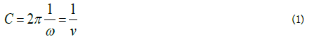
The time circle is tangent to the mathematical timeline at the boundary of the past and future, as Aristotle imagined, and as shown in Figure 1(a). So, it has one measurable point on the timeline but can have a defined duration. The duration we envisioned as a TimePoint (TP) on the circumference of the time circle; we further imagine (TP) traveling continually around the circle, never beginning, never-ending, at a constant rate independent of anything external, as Newton imagined for the flow of time. Still, the TP is different from the flow of time but provides the motion important to Aristotle’s philosophy. Being an abstract item, the movement of the TP is not measurable except for the single boundary point where it couples with mathematical time, the measurable world. The period of the TP defines the minimum possible physical duration and controls the tick rate of attached clocks. Einstein imagined there exists for individuals an I-time or subjective time. These times are not measurable. In that respect, Einstein’s I-time and the NOW are the same; they are not measurable, with the single point exception [13]. This configuration of physical time satisfies both Aristotle’s and Thomas Aquinas’s philosophies.
The configuration of NOW time, as seen in Figure 1(a), has a twofold symmetry, that allows for time reversal. The time circle and the TP are constant and unchanged, never beginning and never-ending; thus, it cannot be reversed. However, without altering its operation, we imagine the NOW time circle shifted to the position seen in Figure 1(b) and pushed whatever has been experienced during its period onto the Future, as depicted by the TP arrow, thus moving time backward (This has an effect on antimatter; Feynman ref. and Stueckelberg ref. have interpreted antimatter and matter as being identical, except antimatter moves backward in time [15,16]. Figures 1(a) and 1(b) suggest that when matter and antimatter come into contact, thus becoming one entity, the Past and the Future are the same, and thus the combined NOW ceases since time cannot stand still, so the physical objects cease to exist. What is measurable is a photon, or equivalent, that carries away the energy and momentum with its own NOW moving forward in time.)

Figure 1: The time circle has duration yet has only one point on the past and future mathematical line. The constant rate of the TP never begins or ends. What physically happens during the NOWâ??s period remains abstract until the TP reaches the boundary point, BP, then becomes measurable and is moved into the past of mathematical time as shown in 1(a).
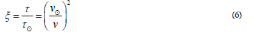
The circumference of the time circle is defined, in (1), by a frequency, so the minimum physical period of the NOW can change due to the influence of external physical frequencies. What frequency does Nature use? Nature has an infinite variety of frequencies, but all are intimately related to compound quantities in space-time, such as the speed of light, momentum, and energy; they are not part of timespace.
Nature has one frequency removed from space-time quantities; the number of photon quanta, a unit-less number, that flows from bright objects and has a unique frequency for each bright source. The number of photons is a multi-valued function of frequency. However, there is one point, or frequency, at which the number of photons is unique, that is, the peak frequency of a Spectral Energy Distribution (SED), at a given temperature. Therefore, we argue that the peak frequency of the SED determines the local flow rate by changing the time duration of the circumference of the time circle, measured in seconds.
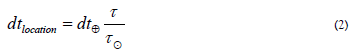
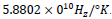
Since the rate of the TP is constant, the period of the NOW changes as a time circle experiences the light of bright sources. In this implementation, the rate of the flow of time on Earth depends upon the SED for the Sun’s surface temperature. On Earth, the peak frequency of the SED of the Sun is  , and the minimum physical period of the TP is
  seconds. With this definition, we can now define a relative flow of time. The Sun is the reference to the time flow anywhere in the universe. It is reasonable since all known physics, theories, experiments, and observations are at a constant flow rate in the Solar system. We measure the Astrophysical or Cosmological properties of the universe from Earth. It is necessary to know the NOW time flow at the distant location. The Transformation Factor (TFF) is the effective temperature of the closest or brightest SED at the studied location. Since the NOW represents a minimum physical time τ. Then in the application of measurements or theories, the differential of time is the essential link to measurable physics at distant locations, so
Where  is in the Sun system and
  measured on Earth, whereas τ is the physical period of the NOW at the distant location of interest, the flow rate of time,
  at the different locations, is referenced to the flow rate in the Sun system. Life forms on systems around different stars will have a different
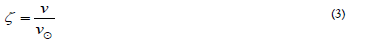
Where v = τ-1 and is the peak frequency of a SED at the location understudy and referenced to the SED peak frequency of the Sun. Determining the minimum duration τ at another location, the circumference of the time circle (1), is involved.
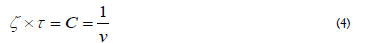
so that
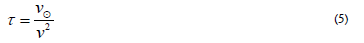
Then the transformation period τ becomes
The transformation is as follows when transforming time derivatives: for physical calculations, the time derivative cannot be carried to the limit of dt →0, as taught in mathematics. Physical calculations must define at dt→ τ . Therefore, in physical calculation time derivatives, we have
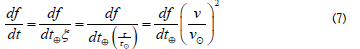
However, as discussed above, all physics is developed on Earth. Therefore, multiplying the transformation (6) by the time differentials translates the time flow rate on Earth to the flow rate at the locations where the action is taking place. When the observed action occurs on Earth,  as seen from (6). Based on the Effective temperature of the distant SED, the peak frequency is
 .
.
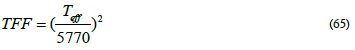
Which then defines a transformation factor TFF as
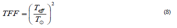
Teff is the best estimate of the SED temperature of distant bright bodies, and TFF is the relative flow of time at a distant location with respect to the flow of time on Earth.
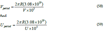
Finally, Newton’s mathematical time, t, can be recovered from this implementation of physical time; with one difference, the flow of time is no longer independent of external influences. Counting the number of rotations, n, of the TP each time it passes the tangent point, the TP becomes the pendulum of all clocks in the solar system and, by transformation, to all clocks anywhere in the universe. Newton’s mathematical time in the Sun system is

So, in practice t = n2.943×10-15 seconds on Earth. During a 24-hour day, the TP rotates 2.936 ×10¹⁹ times. Finally, substituting physical time (9) into spacetime, nothing in physics changes in the solar system. However, in the cosmos, many of the unexplained effects disappear.
1.3 What happens as the TP travels on the time circle, and how long is the NOW
During the TP’s travel, starting at the boundary point and returning to that point, what is happening is not physical but is abstract. Then when the TP completes the circuit and reaches the boundary point, the abstract memory becomes real memory and is “pushed” onto the Past timeline, as depicted by the arrow shown in Figure 1(a).
1.3.1The length of the NOW can be explained by two examples: Example1: Imagine two people are communicating on the telephone. The conversation begins when the TP is at the tangent point on their respective time circles. For both parties, the NOW exists. At the end of each circuit, that part of the conversation enters the physical past timeline for each party, and the conversation continues. The NOW continues as long as the conversation continues. The conversation ends when the TP is at the tangent point; at this point, the conversation has wholly flowed into the past timeline for both parties. If the parties are far apart, there will be silent spaces in the past timeline for as long as it takes light to traverse the distance.
Example2: NOW “recording” events that do not involve conscious beings. Imagine a comet impacting the Earth; as discuss above [2]. The “Earth’s NOW” begins upon impact and continues uninterrupted, constantly passing information from the NOW to past time, as long as the collision’s debris settles on the Earth. Being an abstraction, the NOW can be associated with any physical entity, in this case, the geology of the entire Earth.
1.4 Locating a time circle in space
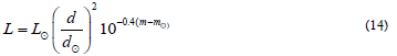
To locate the time circle in space. Equation (9) defines Newton’s recovered mathematical time, so spacetime still applies. Spacetime is unaltered with one exception as the timeline moves through space, the brightness at each point can change; thus, the time flow rate can change along its path. Determining a time circle at a distant location requires a theoretical model. The model allows the user to determine the brightness that affects the particular NOW. The NOW does not require the model; it simply responds to the brightness. The theoretician can use astronomical magnitude calculations.
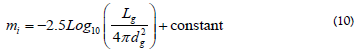
Here Lg is the luminosity of that bright source, and the distance dg is from the bright source to the NOW of interest. In theory, the user can determine the flow rate for any location in space-time. The astronomical apparent magnitudes are employed, and the sum of all bright objects in the universe gives the magnitude m at the point of interest.
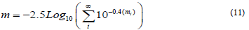
Which generally will reduce to one or a few terms; in practice, we choose a few of the closest bright objects. The user compares the Sun’s apparent magnitude to the apparent magnitude mi for each source.
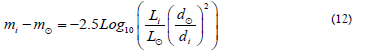
Where Li is the luminosity of the ith distant bright object and di is the distance from the ith bright object to the NOW of interest. Then the magnitude m in (11), determines the peak frequency of the effective SED and, thus, the flow of time at that location given by
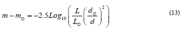
The distance  is the distance from the Earth to the Sun, and d is the distance from the Earth to the location of the NOW, i.e., the luminosity that determines the rate of time is then given by
Then the temperature Teff of the effective SED represented by m is

The radius rs is the effective radius of a sphere that encloses the bright object, and σ is the Stefan-Boltzmann constant.
With physical time defined, we now focus on apparent anomalous effects in current cosmological models.
2. Theories Affected by Time Flow In this section, we look at all the theories that involve time derivatives.
2.1 Classical Electrodynamics
Consider Maxwell’s equation in free space [6]
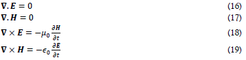
Both Faraday’s law and Ampere’s law involve time derivatives. Therefore, according to (7), the flow of time will influence them. The NOW affects the two equations with time derivatives. These equations are transformed to the distant location and given by
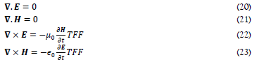
Since the fields E and H are assumed to be abstract quantities as discussed in ref, once the differential equation establishes the fields, they cannot be altered until they undergo another interaction, i.e., E and H cannot be measured until they are part of the measurable universe by combining them in some way with measurable quantities [3]. The mathematical transformation being part of the measurable universe can only affect physically measurable quantities. Therefore, the transformations affect the physical constants, permittivity ε0, and permeability μ0, not the fields in (22) and (23). Therefore, we get
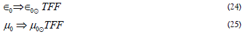
It then follows that the speed of light at the distant location is modified from the value measured in the solar system as follows
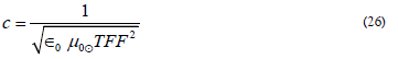
With the introduction of the NOW of time, the speed of light is not a universal constant
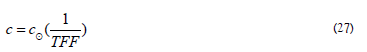
It depends on the local flow of time and can change continuously along the timeline in space-time, depending on the universal brightness at each point.
2.1.1 An example of the rate of a photon traveling from a distant galaxy to Earth: Current physics assumes that the speed of light is a universal constant. Physical time suggests otherwise, as seen in (27). Along its path, the photon and the local NOW move together. Thus, the speed of light varies. Figure 2 shows an example where a photon leaves a distant galaxy, and travels in a straight line to Earth,100 Mpc away The speed of light at the emission point is 1.74 × 10¹⁴ m/s at emission. As the photon progresses, the effect of the galaxy diminishes, and the effect of the Sun increases as indicated by (11), giving a value of 1.74 × 10¹² m/s at the halfway point and the expected value at the Sun-Earth system. All bright sources influence the photon, but only the closest significantly influence the speed of light (Should superluminal phenomena exist and not violate causality, how they would be affected by the NOW of time is unknown; such speculation is beyond the scope of this work) [17].

Figure 2:The variation of the speed of light at different points along its path. The emission point is 100 Mpc from the Earth. In this calculation, the brightness seen by the photon’s NOW combines the emission galaxy and the sun and changes along the photon’s path to the Earth. The emitting galaxy is assumed to have a radius of 20 Kpc and a luminosity of 2.9 × 10¹⁰ times the Sun’s 
2.2 Quantum mechanics and the energy of atomic elements
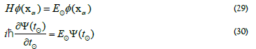
The wave function in Schrodinger’s equation ref is time dependent and given by [8,3]
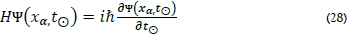
Where H is the Hamiltonian of the system and  is the wavefunction as a function of space
  and mathematical time
  and
and  is Planck’s constant. The time dependence can be removed by defining
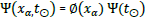
Then (28) becomes two equations
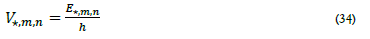
When an atomic system at a distant location is observed, the time derivative (30) is transformed to the location yielding
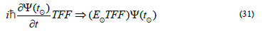
As noted above, since the wave function is a probability amplitude field, it is an abstract quantity [8, 3]. The transformations are only applied to measurable quantities. Therefore, the energy is transformed. The energy levels of atomic elements at the distant location are
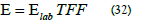
2.3 RedShift determined from atomic spectra
A redshift is essential for studying the universe. If the quantum energy levels are different at distant locations, the RedShift will also be different. When spectral lines are observed and measured, the observed frequency, or wavelength, is evaluated against the emission of the line observed on Earth, usually called the rest-frame frequency or wavelength. The NOW theory provides a means to distinguish possible discordant effects from Doppler effects.
Atomic transitions from state m to state n, using (32) is
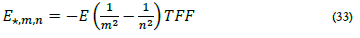
Where E contains only the fundamental constants and m > n. The frequency of the emitted photon at the distant location is
Therefore, the redshift z for the distant spectra is
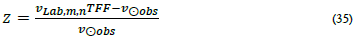
and  is the frequency of the same spectral emission line on Earth; this gives
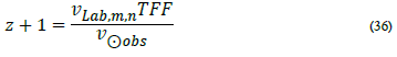
The emission frequency is distant, but the observed frequency is measured on Earth. Therefore, the Transform factor can be obtained from the Redshift, and frequencies measured on Earth are related to the RedShift frequencies measured on Earth. Then the effective temperature Teff and the radiating object’s luminosity, L, are directly measured from the Redshift.
where a is the area of the radiating object and σ is the Stefan Boltzmann constant.
2.4 Special relativity
The NOW will affect the Lorentz equation in Special relativity and General relativity since relative velocity and the speed of light are involved in both [7]. In Special relativity, the gamma factor becomes
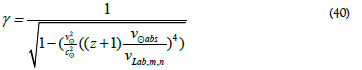
Where the velocity v is measured from Earth but is physically occurring at a distant location. The Lorentz transformations viewed near a distant star become
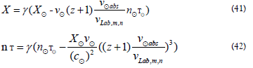
 are the space coordinates measured in the Earth reference frame and X is in a reference frame at the distant location. Similarly, n is the number of complete rotations of the TP, and τ is the period of the TP at the respective reference frame, the velocity
  measured on Earth.
2.5 General relativity
The line element when the speed of light is explicitly shown in the time term, is unchanged at all distances [7,9]. This happens because the correction to the speed of light comes from the permittivity and permeability, shown in (24) and (25), which cancels the transformation for the time differential. Furthermore, time used in general relativity is Newton’s mathematical time measured by clocks, as given in (9), therefore,
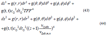
If the line element is written as the proper time dτ2 then the time flow is visible in the line element
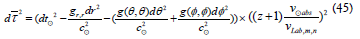
Consider, for example, the Schwarzschild solution
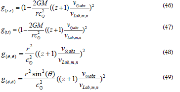
The metric tensors are corrected for the speed of light.
2.6 Redshift determined from Cosmological considerations To examine the expansion of space, the Robertson-Walker metric is used [18]

Where a is the scale factor, the Earth-bound observer is at r = 0 and at mathematical time t = tthen , observing the crest of light waves emitted at the distant location and mathematical time r = R and t = tthen. This calculation assumes the expansion is only along the radial direction with the Sun at the origin, neglecting the slight Sun-toEarth difference. For light, the physical time of emission is at the boundary point at that location and set to zero, i.e., dτ = 0. To trace the wave crest, Integrating (49) yields [18]
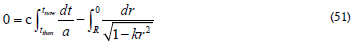
When the light was emitted t = tthen + λthen/cthen, the next wave crest seen by the observer is t = tnow + λnow/cnowthen
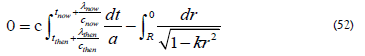
Subtracting (50) and (51) gives
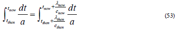
The result allowing for the correct speed of light gives
Where cnow =  and cthen = ;TFF−1, and the factor αthen is the scale at the distant location, and anow is the scale at the Earth. Then
therefore,

The factor αthen is the scale at the distant location, whereas the αthen is the scale at the Earth. Therefore, αthen = 1 and then αthen = (z + 1)−1TFF.
Part 2
3. Galaxy rotation
The rotation velocity of the galaxies does not decrease with stars’ orbit distance from the center, as gravitation theories predict, but remains constant with radial distance. Zwicky [19] observed this while studying nebulas, and he argued that the fast rotation meant the stars would attain escape velocity, and thus nebulae could not exist, so there must be more mass than observed. This unseen mass became known as dark matter because it does not emit radiation and only interacts with gravitation. Rubin ref studied numerous galaxies and found they all behave similarly, exhibiting a flat rotation curve [20].
These observations have led to a century-long search for properties of dark matter. The dark matter could be dead stars, escaped planets, perhaps black holes, or a new subatomic particle, but nothing has been found. There also have been efforts to modify gravitation theory to explain the unusual rotation. Modified Newtonian Mechanics, MOND developed by Milgrom ref, has been found to reproduce the flat rotation curve measured for all galaxies but requires an extra adjustable parameter [21]. Gravitomagnetic by Ludwig fits the rotation curves but fails to produce the luminosity profile, and the disk fails to give its mass distribution and total mass [22]. There needs to be a satisfactory explanation of the dark matter.
Andromeda, our closest galactic neighbor, will be used to discuss the effect of the NOW’s physical time’s impact on galactic rotation because its measured properties, rotational velocity, and detailed photometry are well established. Rubin ref measured the rotation curve and found the curve to be flat, as opposed to that expected by gravitation theory [23,24]. De Vancouleur’s ref photometry measurements of Andromeda are detailed compared to more distant galaxies.
3.1 Rotation data and analysisThe data used in the analysis of Andromeda are given in the three (Tables 1-4 and Figure 3). We take the nuclear region from the center to 8kpc and the disk region from 8kpc to 30kpc. These boundary conditions for the start and end of the disk are determined by the peak velocity in the fit to measured rotation data, seen in Figure 4, and the limit of visible matter, about 30kpc. This demonstration will be limited to the disk region since this disk region is where the gravitational predictions are the most pronounced. Rubin’s disk region, ending at 27.5Kpc, is extended to 30Kpc, with measurements by (Roberts, Whitehurst) ref, to prevent the polynomial fit of Rubin’s rotation velocity Vrot data from diverging prematurely [25].
TABLE 1. Andromeda measured data. De Vancouleurs Position along the semi-major axis in kpc given in column1 and column 2 the brightness, Square Arc-Sec (SAS). Rubins rotational velocity in column 3
| R | σL | Vrot |
|---|---|---|
| Kpc | LSun/SAS | Km/sec |
| 1 | 2 | 3 |
| 2.75 | 1360 | 196.3 |
| 5.5 | 615 | 248.8 |
| 8.25 | 530 | 264.5 |
| 11.0 | 270 | 261.1 |
| 16.5 | 70 | 239.2 |
| 22.0 | 20 | 228.0 |
| 27.5 | 5.5 | 230.0 |
| 30.0 | --- | 230.0 |
TABLE 2. Conversion of SAS to pc2 . Kpc position, mass density per SAS, mass density per pc2 , and the ratio of minor to major axis, are given in columns, 1,2,3,4 respectively, in column 5 the conversion pc2 /SAS
| R | σLsun/pc2 | Lum (1038) | (T/TSun )2 | Urot |
|---|---|---|---|---|
| Kpc | LSun /pc2 | watt | TFF | Km/sec |
| 1 | 2 | 3 | 4 | 5 |
| 2.75 | 147.2 | 221.1 | 0.548 | 107.6 |
| 5.5 | 66.6 | 99.9 | 0.390 | 97.0 |
| 8.25 | 57.2 | 86.2 | 0.278 | 73.5 |
| 11.0 | 29.2 | 43.9 | 0.199 | 52.0 |
| 16.5 | 7.60 | 11.4 | 0.102 | 24.4 |
| 22.0 | 2.20 | 3.3 | 0.053 | 12.1 |
| 27.5 | 0.60 | 0.9 | 0.029 | 6.67 |
| 30.0 | 0.60 | --- | 0.022 | 5.06 |
TABLE 3. Conversion of Rotation velocity. Kpc, Brightness/pc2, Luminosity, TFF, in columns 1, 2, 3, 4, respectively. Column 5 transformed rotation velocities in Km/sec
| R | σLsun/pc2 | Lum (1038) | (T/TSun )2 | Urot |
|---|---|---|---|---|
| Kpc | LSun /pc2 | watt | TFF | Km/sec |
| 1 | 2 | 3 | 4 | 5 |
| 2.75 | 147.2 | 221.1 | 0.548 | 107.6 |
| 5.5 | 66.6 | 99.9 | 0.390 | 97.0 |
| 8.25 | 57.2 | 86.2 | 0.278 | 73.5 |
| 11.0 | 29.2 | 43.9 | 0.199 | 52.0 |
| 16.5 | 7.60 | 11.4 | 0.102 | 24.4 |
| 22.0 | 2.20 | 3.3 | 0.053 | 12.1 |
| 27.5 | 0.60 | 0.9 | 0.029 | 6.67 |
| 30.0 | 0.60 | --- | 0.022 | 5.06 |
TABLE 4. Hubble’s law with respect to the NOW time
| NGC | D | D0 | nLn | Z |
|---|---|---|---|---|
| --- | Mpc | Kpc | LSun-loboΧ1010 | --- |
| 196 | 58.3 | 22.3 | 1.85 | 0.01319 |
| 331 | 70.4 | 29.8 | 2.97 | 0.01649 |
| 315 | 55.1 | 48.9 | 10.7 | 0.01648 |
| 410 | 62.5 | 39.3 | 10.8 | 0.01736 |
| 426 | 128 | 46.9 | 0.633 | 0.00760 |
| 502 | 33.8 | 11.2 | 0.633 | 0.00760 |
| 529 | 52.5 | 37.0 | 4.57 | 0.01190 |
| 661 | 27.4 | 14.4 | 1.71 | 0.00620 |
| 665 | 47.1 | 31.7 | 3.66 | 0.01822 |
| 677 | 67.0 | 41.1 | 3.36 | 0.01693 |
| 777 | 53.0 | 37.3 | 8.57 | 0.01673 |
| 794 | 113 | 42.3 | 8.80 | 0.02560 |
| 990 | 42.4 | 23.8 | 1.72 | 0.01319 |
| 1004 | 88.4 | 28.74 | 4.14 | 0.02159 |
| 1016 | 58.0 | 22.89 | 9.40 | 0.01210 |
| 1060 | 61.3 | 45.2 | 10.1 | 0.01390 |
| 1101 | 81.7 | 31.1 | 3.07 | 0.01850 |
| 1107 | 40.8 | 22.9 | 1.73 | 0.01107 |
| 1132 | 85.4 | 54.6 | 6.54 | 0.02313 |
| 1201 | 20.2 | 19.6 | 1.15 | 0.00562 |
| 196 | 63.85 | 23.1 | 1.85 | 0.01414 |
| 471 | 62.34 | 17.9 | 1.09 | 0.01375 |
| 1008 | 96.64 | 20.9 | 1.29 | 0.02179 |
| 1132 | 102.26 | 65.1 | 6.54 | 0.02313 |
| 2713 | 55.27 | 60.3 | 11.3 | 0.01299 |
| 3106 | 90.76 | 47.1 | 3.03 | 0.02065 |
| 3710 | 94.46 | 8.8 | 0.421 | 0.00436 |
| 3838 | 20.54 | 22.9 | 1.73 | 0.01107 |
| 5332 | 99.18 | 25.1 | 5.36 | 0.02240 |
| 6003 | 61.01 | 16.3 | 0.993 | 0.01350 |
| 6560 | 106.88 | 37.3 | 2.58 | 0.02349 |
| 7580 | 67.86 | 15.8 | 1.33 | 0.01480 |
| 7624 | 65.87 | 19.3 | 1.97 | 0.01426 |
| 7625 | 26.55 | 12.1 | 1.54 | 0.00543 |

Figure 3: The transformation factor is given in Table 3, column 4 for each as a function of R Kpc column 1 measured value. The disk portion of Andromeda is fit to an exponential 0.0035 + 0.7665e−0.1243R, which is utilized in converting Rubin’s rotation velocities

Figure 4:Measured Vrot Black, NOW corrected Urot, Red. The black points are Rubins measured rotational velocities, the open data points are the extension to the measured data as described in the text. The Red points are the transformed point using the exponential fit given in Figure 3. The fit to the transformed velocities, red points, has the expected gravitational functional form  the constant is the rate of the entire galaxy moving toward the Milky Way; see the text for more details
A transformation factor, discussed in section 2.2, is applied to rotational Vrot to apply this NOW theory to the galaxy rotation. De Vancouleurs measured the B surface brightness in each squared arcseconds (SAS) region along the semi-major axis as a function of the distance from the galactic center in Kpc, given in Table 1, columns 1, the isophotes distance from the center, expressed in Kpc, and column 2, expressed in units of solar units per SAS. Each unit’s contribution to the luminosity is from the stars within the boundary of the SAS unit. The space in the unit contributes nothing to the luminosity but to the densities if needed. To account for the space between stars in the SAS, the SAS is converted to pc2 . De Vancourleurs provides the mass density in both SAS and pc2 . The mass densities σM and σ’M given by De Vancouleurs and included in Table 2 for both SAS and pc2 .
Thus, the ratio of the mass density accounts for the space in each unit. Therefore, the brightness conversion in Table 3 accounts for the space in the density calculations but contributes nothing to the luminosity. The conversion factor was obtained from (de Vancouleurs [24], Table 5, using columns 2, 3, 5, and 6) and shown in the first four columns in Table 2. When averaged over all isophotes, the result in column 5 yields the conversion, 9.24 ± 0.48 pc2 /SAS.Rubin [23] indicates a typical Stromgren sphere [26] in Andromeda, which is the spherical influence of a star, appears to be several seconds of arc in diameter. The temperature of the star obtained from (15). with the radius of the Stromgren adopted to be rs = 1.5pc as suggested by Rubin.
TABLE 5. Hubble’s constant at three Mpc distances from Earth.
| R | Hubble | Hubble 10-10 |
|---|---|---|
| Mpc | As measured | NOW corrected |
| 1 | 2 | 3 |
| 10 | 68.75 | 0.943 |
| 60 | 74.14 | 1.399 |
| 120 | 65.66 | 0.478 |
Luminosity and temperature from Photoelectric Photometry measurements of Andromeda Galaxy are obtained from de Vancouleurs and given in Table 3 in columns 1 and 2. These are the primary brightness data measured along the semi-major axes from the galaxy’s center. The luminosity and the transforming factor are in columns 3 and 4, respectively. The measured rotation velocity, Vrot, in column 3, in Table 1, is from Rubin’s Table 1, and the time flow corrected rotation velocity, Urot, given in column 5 of Table 3. The entries for Vrot and Urot were obtained as discussed in the text.
The resulting calculations are given in Table 3, column 5, and shown in Figure 4, where the NOW corrected rotation velocities Urot for the disk region are shown in red. The best fit to the NOW corrected rotation velocity is
The red points in Figure 4 clearly show the correct gravitational behavior and the magnitude of the corrected rotation velocities is determined by the value of rs the Stromgren radius.
The black dots are the directly measured rotation velocity from Rubin’s Table 1, and the open black circles are extended points discussed in the text. A 6th-order polynomial best fits the measured data, shown as a solid brown curve in Figure 4. The red dots are the point-for-point transformed rotation velocity described in the text.
The brown curve best fits the transformed population in the disk region. As can be seen, the fitting function has the expected gravitational dependence  − 72.08, where −72.08 km/sec and represents the entire galaxy velocity moving toward the Milky Way. To see that the fit to the entire rotation produces the expected rotation and a linear velocity of −72.08 km/sec. The measured velocity of the entire M31 galaxy moving toward the Milky Way is −130 km/sec. When this is transformed, by 0.548, from Table 3 column 4, which is the only measured velocity undergoing minimal rotation, we get −71.24 km/sec. Close to the fit constant. 4.2 Mass of And
3.2 Mass of andromeda
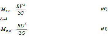
The mass is determined from Rubin ref and De Vaucouleurs Isophote data [23,24]. Each Isophote has a unique rotation velocity, both as measured and after NOW transformed. Since each Isophote is consistent with the gravitation theory, as shown in Figure 4. The period of rotation of each Isophote is determined,
Where R from either Table 1, 2 or 3 Column 1, V in units of meter per second from Column 3 of Table 1, and U in units of meter per second from Column 5 of Table 3. These results are given in Figure 5.

Figure 5: The Log of the rotation period as a function of each Isophote, shown in blue for the as-measured velocities and red for the NOW transformed velocities
From gravitational energy (1/2)mV2 = GMm/R, the mass associated with each Isophote is given by
The total mass of M31 is
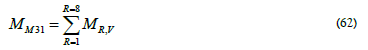
MM31 = 6.82 × 10¹¹Suns, with velocity as measured. This value includes dark matter since the velocity curve is flat in the disk. The NOW corrected velocity, which responds as expected from gravity theory, does not have dark matter and is given by
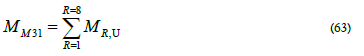
which is MM31 = 5.2 × 10⁹ Suns with velocity NOW transformed
4. Hubble’s law
Einstein’s general relativity has a time-dependent solution that surprised its creator, whose philosophy was a forever unchanging universe. To overcome the time-dependent solution, Einstein modified general relativity by adding a term he called the cosmological constant designed to remove the time-dependent solutions. When Hubble’s observation ref provided evidence that the universe was expanding, Einstein regretted the modification [27]. Hubble’s law and the time solution to GR suggested to Lemaitre ref that the universe must have been microscopic in the distant past [28]. All the matter in the universe would come to a single point, containing the universe’s total energy, and explodes forth, creating space, time, and the universe; this is now called the Big Bang. The first few moments of the universe must have been very hot, and as it expanded, it cooled, giving rise to a radiation field known today as the Cosmic Microwave Background (CMB). The CMB is thought to be the most substantial supporting evidence for the Big Bang. The Big Bang is a speculative idea based on Hubble’s measurements by running Newton’s mathematical time backward, even though no clocks can measure the progress. Once the Big Bang is established, the CMB naturally follows from the expansion. The CMB is thought to be a thermodynamic cooling effect based on speculation about the measured expanding universe.
To re-investigate Hubble’s law with respect to the NOW time, I chose to use only the brightest galaxies, given by Frueh et al [29]. That work studied the “Photoelectric UBV Photometry of 179 Bright Galaxies. The criterion for the 34 galaxies list in Table 4 was also available in the NED IPAC database [30]. This ensured that all the measured parameters needed to implement the NOW time transfer factor, TFF were available for each galaxy. The data used in this analysis are given in Table 4.
The velocities of the selected bright galaxies are obtained from the redshift v = z × c, and the best fit shows a slight downward-opening parabolic curve seen in Figure 6. A straight line fit to this data has an offset at the origin of 500.6 km sec−1 , and a Hubble constant is H0 = 64.2km sec−1 Mpc−1 , suggesting the fit is a higher order then one. The offset at the origin is not observed in Hubble’s data. When a square term is allowed, and as seen in the fit, Figure 6 results and brings the origin value to −31.9km/sec, near zero, as expected. The best fit is a parabola opening downward, as can also be seen in Figure 6. The Hubble Constant slowly changes with distance. The changes in the Hubble constant are given in Table 5, columns 1 and 2 in units of km sec−1 Mpc−1 To determine the effect of the NOW time the transform factor TFF is first determined. Equation (15) determines the temperature and (8) determines TFF. The effective temperature, uses the galaxy’s luminosity and radius, the radius of the galaxy is half of the semi-axes R = D0/2 given in Table 4, and the effective temperature of each galaxy is obtained by
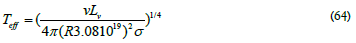

Figure 6:The red dots with x-y standard deviation bars were obtained by a running average of two successive values. The red dots are the averaged points. The original points were obtained by v = z × c versus Mpc. The speed of light is assumed to be constant for this calculation. The best fit is a slightdownward-opening parabola
where σ is the Stefan- Boltzmann constant. The transform factor, TFF, is then
To determine how to make the NOW corrections, we start with the Robertson-Walker metric (50) and factor the dt2 term because we are interested in the velocity as opposed to the gravitation effects, thus
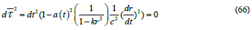
For a photon  then it follows,
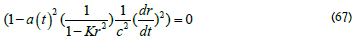
Solving this for the velocity factor V /c. The speed of light (27) and time derivative (7) must be correct for the NOW time. The transformed TFF enters twice,
Where the velocity  , is the Hubble measured velocity shown in Figure 6 and the NOW corrected velocity U is

The effect of the NOW time is obtained by multiplying each velocity point in Figure 6 by the TFF2 to obtain the NOW corrected velocities U, and are shown in Figure 7.

Figure 7: The Hubble’s expansion is reduced by about 12 orders of magnitude from the Hubble measured values, and the downward opening parabola is accentuated by the NOW time correction.
Table 5, columns 1 and 3. gives the Hubble Constant in units of km sec−1 Mpc−1 after the NOW time correction. The velocities U are twelve orders of magnitude slower than Hubble measured, which suggests the big bang did not happen as thought, and suggests a different structure of the universe. Its downward progression is a strong argument against an accelerating universe and dark energy and will easily account for the distant galaxy observed by the James Webb Space Telescope. If the Big Bang did not happen, then what is the CMB?
4.1 New interpretation of the CMB
The CMB SED spectrum indicates that an Energy density u exits everywhere in the universe. The energy density is obtained from the SED spectrum by dividing it by the speed of light. The mean temperature of the CMB is 2.726K. Thus, the energy density is
For this speculation, the constant Earth value of the speed of light will be used. Whereas for a detailed calculation of distant galaxies, the transformed speed of light would need to be used. It is well known, from thermodynamics and from Einstein’s, E = mc2 , that energy does not have a fixed “form” [7]. It can change if the effective amount remains constant. For example, potential energy can be converted to kinetic energy and kinetic energy to heat energy. This new interpretation of the CMB postulates that the CMB energy (69) is converted to the Hydrogen atom’s mass-energy. The physics of CMB energy conversion will be left for future study
The energy of the Hydrogen atom is EH = 938.8 × 10⁶ ev/H = 1.504 × 10⁻¹⁰ joule/H. Using (69), this equals EH/u = 1.418 × 10⁴ meter3 /H. For this calculation, it is assumed that TFF ≈ 1, so the c = in (69). With this approximation, the Milky Way estimates the hydrogen production rate. For example; the Milky Way volume at about 1.7 × 10¹³ Lyr3 , or 1.44 × 1061 meter3 which we adopt. This indicates sufficient energy to yield approximately 1.0 × 1057Hatoms and thus a mass production is 1.67 × 10⁻²⁷ kgm/Hatom × 1.0 × 1057Hatoms = 1.7 × 1030 kgm which is, within the approximation, the mass of the Sun. How long does it take to produce this mass? The estimated star production rate in the Milky Way [31] is approximately one Sun every half year, about 183days, which requires 1.0 × 1057Hatoms/183 days. Therefore, the vacuum energy in the Milky Way is sufficient within the confines of the Milky Way to produce two suns each year.
The replenishment of Hydrogen in galaxies happens randomly throughout the universe and, over long periods, newly created hydrogen migrates into clouds within which stars are formed.
A similar process is happening in all galaxies throughout the universe. Therefore, Hydrogen is being replenished continuously everywhere in the universe. If hydrogen replenishment were not available, the universe would slowly grow dark and end as a dark cinder of the heavier elements, which forms as the stars live and die.
Hydrogen replenishment in galaxies happens randomly throughout the universe and, over long periods, newly created Hydrogen migrates into clouds within which stars are formed. A similar process is happening in all galaxies throughout the universe. Therefore, Hydrogen is being replenished continuously everywhere in the universe. If the universe is finite, Energy taken from the CMB reduces the energy density, thus lowering the CMB energy content. In a finite steady-state universe that is eternal, this process continues forever. Hence the CMB must recover the lost Energy. This recovery could be continuous from the quantum zero-point energy or the cosmological constant [32].
Another possibility; is if an infinite steady-state universe is envisioned. It can be argued that removing finite amounts of energy from the infinite CMB does not alter the “infinite status” of the CMB; it remains infinite. Thus, there is an eternal process of life and death of stars in the universe instead of an initial beginning and ultimate death; therefore, the universe is continually being created by its eternal maintenance. In time, the contribution of Hydrogen from the CMB maintains existing galaxies and creates new galaxies by creation in intergalactic space.
In this interpretation of the CMB, one can entertain the philosophy that with the eternal increase of stars and galaxies, an increase in planets will soak up the ever-increasing heavy elements and eternal increase in life forms, thus maintaining an even balance of atomic elements.
Criticisms of the Big Bang can also apply to this speculation. However, there is one main difference, the CMB is directly measurable, whereas the Big Bang is not. So, we conclude that the universe is continuously being created by its maintenance from the vacuum energy. It did not exist in one big flash and would not end in a whimper. Those who prefer to imagine an infinite and eternal divinity that created the universe can imagine the eternal divinity forever, creating and maintaining the universe.
5. Pioneer anomaly
Another anomaly within the Sun’s system: The Pioneer 10 and 11 Spacecraft (SC) were designed to probe the outer planets of our solar system. In 1998, Anderson reported that when the solar radiation pressure had decreased sufficiently at about 20 AU from the Sun, an unexpected constant acceleration of (8±3) ×10−10 m/s2 directed toward the Sun was found to be the most significant systematic error [33-35].
There have been many attempts to explain the anomaly, ranging from new physics to engineering anomalies on the spacecraft. Dittus ref and Turyshev ref and references therein reexamine all measured data from Pioneer’s mission [36,37]. Anderson ref critiqued many possible explanations; see the references therein [38]. This section adds to the new physics category as a possible explanation; It can be explained by the introduction of the NOW time.
To obtain Doppler data for the Pioneer SC, the Deep Space Network (DSN) was used to send a reference frequency to the SC that was then sent back to the DSN by an onboard transponder. This allowed detailed tracking of the SC.
5.1 Implementation
The SC is tracked through the Deep Space Network (DSN), where reference frequency is sent to the SC and then returned to the DSN by the SC. That data is compared to the theoretical calculation of the SC position and velocity. If they match, then

If we know all effects that influence the SC, we can set the SC returned frequency, vobs(t) = vmodel(t) . However, if the observing vmodel(t) is not correct, let us write vobs(t) =  (t) ,where
  model(t) is the observed frequency in which something is missing, this is indicated by a ~ over a quantity. Then (70) can be written in terms of an unknown acceleration integrated over time
where the Doppler frequency is given by
Inserting (72) into (71) yields
The LHS is a quantity at the distant location of the SC, thus needing the NOW correction. The RHS is constructed on Earth after the information is returned to the DSN; the NOW correction factor on Earth is 1 and does not change the quantity. Time, t is the mathematical time Newton defines and determines by a clock; the difference between the Newton-defined time and the NOW-defined time is the clock’s rate. The brightness at the location of the NOW determines the difference. Finally, the anomalous acceleration can be expressed as
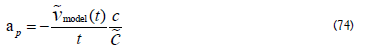
Where expressing  as given in (27). Approaching the problem this way gives the correct sign, i.e., the anomalous acceleration is pointed toward the Sun opposite to the direction the SC travels.
5.2 Applying the NOW theory
In this application, the Sun is unchanging, but we need to know the physical process on a distant SC; thus, the local NOW on the SC needs to be determined compared to the NOW on Earth. This is done using the apparent brightness at the SC compared to the Earth’s value and will be called B instead of TFF since it is due to the change in the distance to the Sun and not due to independent, bright sources. The brightness, as obtained from the Flux, diminishes by the distance from the Sun due to the apparent angular radius of the Sun viewed at a distance of r. The angular radius can be obtained by a ratio of that seen on Earth to that seen at a distance r from the Sun and is given by
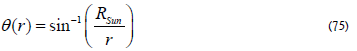
The Sun radius and the distance to the SC are expressed in astronomical units, RSun = 4.7 × 10⁻³ Au; therefore, sin(θ(r)) = (4.7 × 10⁻³ )/r. The Flux from the Sun at a distance r is obtained from the intensity, Iν, which is the SED of the Sun, by integrating the solid angle

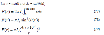
The intensity Iν is an intrinsic property of the Sun and does not depend on distance. Therefore, the intensity cancels out when the relative brightness B, is formed,
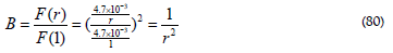
F(1) is the Flux on Earth at 1Au from the Sun. Applying the transform factor to both the velocity and the speed of light as
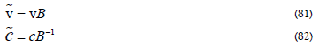
Combining (81) and (82) with (74) gives the final result, which is the anomalous acceleration in the NOW theory of time instead of the Newton theory of time
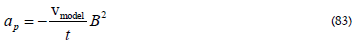
The pioneer 10 data in Table 6 were obtained from HelioWeb [39]. The transform factor for the NOW time theory and the anomalous acceleration is given in Table 7. The average of column 4 of Table 7 gives the value for the anomalous constant acceleration, 7.3 × 10⁻¹⁰ m/sec2 , which compares well with the excepted value of 8. × 10−10 m/sec2 given by Anderson [33]. This can be improved somewhat if we assume a few of the onboard contributions, which seem reasonable, as listed in Table 8, assuming positive values. In that case, they average to 0.82 × 10⁻¹⁰ m/sec2 , thus bringing the total to 8.12 × 10⁻¹⁰ m/sec2 well within the given uncertainty for the anomalous acceleration. Others have considered time, e.g., It was found by Laing, using CHASMP, that a steady frequency drift of about −6 × 10⁻⁹ Hz/sec [40]. Ranada ref has considered time acceleration as a possible answer linking it to the universe expansion [41]. Anderson ref ruled that out because if there were a steady drift in the atomic clocks of the DSN or time reference standard, all clocks would change with constant acceleration [35]. That would be true for Newton’s mathematical time since mathematical time is independent of external influences. In Anderson, a careful look at the graph’s large “day end” shows two small but distinct oscillations, each a year-long, suggesting the Earth’s orbital motion is affecting the result, which is consistent with the NOW time [35-44].
TABLE 6. Data from HelioWeb [39]. The data used in the calculation are: The year is given in column 1, in 2 the interval in days, in column 3 the distance in AU traveled in the time interval distance given in 2, and 4 the time in seconds to travel the distance listed in 3. In column 5, the SC velocity in meters per second, and in column 6 is a measure of anomalous acceleration in the Newtonian time system
| Year | ΔDay | Δr | t | V | V/t |
|---|---|---|---|---|---|
| --- | --- | AU | 106 sec | 104 m/sec | 10-3 m/s2 |
| 1 | 2 | 3 | 4 | 5 | 6 |
| 1985 | 50. | 0.38 | 4.32 | 1.31 | 3.03 |
| 1990 | 50. | 0.36 | 4.32 | 1.25 | 2.89 |
| 1995 | 50. | 0.35 | 4.32 | 1.21 | 2.80 |
| 2000 | 50. | 0.35 | 4.32 | 1.20 | 2.78 |
TABLE 7. Column 1 is the year, 2 is the AU distance from the Sun, and 3 is the transform factor, in column 4 is the anomalous acceleration at each position
| Year | r | B2 | ap = V B2/t |
|---|---|---|---|
| AU | 10-8 | 10-10 m/sec2 | |
| 1 | 2 | 3 | 4 |
| 1985 | 34.68 | 69.14 | 20.94 |
| 1990 | 48.37 | 18.27 | 5.28 |
| 1995 | 61.37 | 7.05 | 1.97 |
| 2000 | 74.52 | 3.24 | 0.901 |
TABLE 8. Effects generated by the operation of the SC that seem most reason- able. Each effect is assumed to contribute a positive effect to the anomalous acceleration
| Onboard Acceleration | 10-10 |
|---|---|
| Radio beam reaction force | 0.11 |
| RTG heat reflected from the SC | 0.55 |
| He expelled from RTG | 0.16 |
If GR equation (43) to (49) were used to develop the position and velocity. the result in table 7 column 4 should be obtained. Therefore, it suggests that the Helioweb data is not correct
Conclusion
The foundation of modern physics was determined by Newton. He defined both space and mathematical time. In this work, we questioned the foundation of both space and time; neither has been reviewed since Newton defined them, even though philosophers have looked for better definitions. Einstein found that space and time are linked into a four-dimensional space called space-time, and due to the speed of light, thought to be a universal constant. Both space and time are measured differently by observers moving relative to each other and or in different gravitational fields. However, observers still use mathematical time read on calibrated and synchronized clocks within each reference frame, as Newton defined. We question if a measure of time defines time and decide it leaves out something meaningful. Newton recognized that time flowed and defined it as a universal constant that is the same everywhere in the universe, but he did not define it. We find that time has the most significant effect on astrophysics and cosmology, so we have concentrated on the definition of time. The space part of the foundation of physics is not included in this work; it has been published elsewhere. Parts of this paper have been published ref, and represent early thoughts.
Over the last century, much work has been done to define and understand the broader universe, and numerous anomalies inconsistent with gravitation theory have been observed. There have been numerous attempts to modify physical theories to make them fit the observations. In this work, we find that the definition of time is the biggest problem; defining a physical time instead of a mathematical time eliminates many of these anomalies. The problem comes down to the interpretation of measurements. With an appropriate definition of physical time, galaxies rotate as expected from existing gravitation theory. The speed of light is not a universal constant as thought. Hubble’s law is modified, which suggests the Big Bang may be just another anomaly, and that suggests the CMB needs to be reinterpreted, which we do. Finally, we find a solution to the Pioneer space-craft anomalous acceleration.
In the introduction of this work, it was said the foundation of physics defined by Newton was responsible for many of the effects in cosmology that are not explained by existing physics. We have shown that a minor change in one property of Nature will explain six independent and previously unexplained phenomena. At first, I thought this was surprising. However, this single property is a significant part of the foundation of all modern physics, science, and civilization.
Time has never been defined; only times measurement has been offered, and measuring any quantity is not a true definition of that quantity. We have seen this with gravity; Newton provided a measure of gravity, its force that moves masses. Einstein showed that energy alters the geometry of space-time and has brought us closer to a definition of gravity. However, we have yet to arrive since gravitation and quantum mechanics still need to be reconciled. However, the space part of the foundation of physics has potentially provided a connection, see Longo ref, which has been published elsewhere and was not considered in this paper ref. Some thoughts on how this theory might be falsified. The results quoted herein are strongly dependent on astronomical measurements. For distant galaxies, it needs to be clarified how the peak of the SED of distant galaxies is determined. If that problem can be solved, the Big Bang, the CMB, and Dark Energy might be revisited. Dark matter is less of a problem, at least for the Andromeda galaxy, because the photometric measurements were more readily attainable and more detailed. One can hope the new James Webb Space Telescope can add photometric clarity for more distant galaxies.
Acknowledgement
The author thanks G.L. Harnagel for many helpful discussions.
References
- Newton I. The Principia: Mathematical Principles of Natural Philosophy. Cohen BI, Whitman A, 1999. [Googlescholar] [Crossref]
- Longo RT. New Trends in Physical Science Research Nuclear Decay Rate Oscillations and a Gravity-Quantum Connection. 2019 [Googlescholar] [Crossref]
- Dyson FT. Why is Maxwell’s theory so hard to understand? [Googlescholar]
- Richard K. Plato. The Stanford Encyclopedia of Philosophy (Spring 2022 Edition). Edward NZ. [Googlescholar]
- Tegmark M. Our Mathematical Universe: My Quest for the Ultimate Nature of Reality by Max Tegmark. ISBN 978-0307599803. [Googlescholar] [Crossref]
- Maxwell JC. A dynamical theory of the electromagnetic field. Philosophical Transactions of the Royal Society of London. 155: 459-512: 1865. [Googlescholar] [Crossref]
- Einstein A, W Perrett, G.B. Jeffery. The Principle of Relativity, On the Electrodynamics of Moving Bodies, and The Foundation of the General Theory of Relativity. Dover Publications, Inc.1895. [Googlescholar]
- Messiah A. Quantum Mechanics. Vol I, Vol II. Northholland Publishing Company, 1961.
- Thorne KS, Wheeler JA, Misner CW. Gravitation. San Francisco, CA: Freeman; 2000.
- Paston SA, Sheykin AA. Embeddings for the Schwarzschild metric: classification and new results. Classical and Quantum Gravity. 2012; 29(9):095022.
- Weidhorn M. The person of the millennium: the unique impact of Galileo on world history. I universe; 2005.
- Muller RA. Now-and the physics of time, Cosmos Culture. 2016.
- Davies P. About Time: Einstein’s Unfinished Revolution, A Touchstone Book. Simon Schuster. 1996.
- Minkowski H, Perrett W, Jeffery GB. Space and Time. Dover Publications, Inc. 1923.
- Feynman RP. Space-time approach to non-relativistic quantum mechanics. Reviews of modern physics. 1948; 20(2):367.
- Stückelberg EC. The meaning of proper time in wave mechanics. Helv. Phys. act. 1941; 14:322-3.
- Harnagel GL, Tachyons. The Four-Momentum Formalism and Simultaneity. Universal Journal of Physics and Application. 17(1): 1-7: 2023.
[Crossref]
- Weinberg S. Gravitation and Cosmology. John Wiley Sons, Inc., 1972.
- Zwicky F. On the Masses of Nebulae and of Clusters of Nebulae. In A Source Book in Astronomy and Astrophysics. Harvard University Press.1937.
- Rubin VC, Ford Jr WK, Thonnard N. Rotational properties of 21 SC galaxies with a large range of luminosities and radii, from NGC 4605/R= 4kpc/to UGC 2885/R= 122 kpc. Astrophysical Journal. 238. 1980; 238:471-87.
- Milgrom M. A modification of the Newtonian dynamics as a possible alternative to the hidden mass hypothesis. Astrophysical Journal. 1983; 270:365-70.
- Ludwig GO. Galactic rotation curve and dark matter according to gravitomagnetic. The European Physical Journal C. 2021; 81(2):1-25.
- Rubin VC, Ford Jr WK. Rotation of the Andromeda nebula from a spectroscopic survey of emission regions. Astrophysical Journal. 1970; 159:379.
- de Vaucouleurs G. Photoelectric photometry of the Andromeda nebula in the UBV system. Astrophysical Journal. 1958; 128:465.
- Roberts MS, Whitehurst RN. The rotation curve and geometry of M31 at large galactocentric distances. Astrophysical Journal. 327-346. 1975; 201:327-46.
- Strömgren B. The physical state of interstellar hydrogen. InA Source Book in Astronomy and Astrophysics. 1979: 588-592. Harvard University Press.
- Hubble E. A relation between distance and radial velocity among extra-galactic nebulae. Proceedings of the national academy of sciences. 1929; 15(3):168-73.
- Lemaître AG. Contributions to a British Association Discussion on the Evolution of the Universe. Nature. 1931; 128(3234):704-6.
- Frueh ML, Corwin Jr HG, De Vaucouleurs G, et al. Photoelectric UBV Photometry of 179 Bright Galaxies. Astronomical Journal. 1996; 111:722.
- The Principia: Mathematical Principles of Natural Philosophy
- Lefebvre-Omar C, Liu E, Dalle C, et al. Neurofilament accumulations in amyotrophic lateral sclerosis patients’ motor neurons impair axonal initial segment integrity. Cellular and Molecular Life Sciences. 2023; 80(6):150.
- Kragh H. Preludes to dark energy: zero-point energy and vacuum speculations. Archive for history of exact sciences. 2012; 66:199-240.
- Anderson JD, Laing PA, Lau EL, et al. Indication, from Pioneer 10/11, Galileo, and Ulysses data, of an apparent anomalous, weak, long-range acceleration. Physical Review Letters. 1998; 81(14):2858.
- Anderson JD, Lau EL, Turyshev SG, et al. Search for a standard explanation of the pioneer anomaly. Modern Physics Letters A. 2002; 17(14):875-85.
- Anderson JD, Laing PA, Lau EL, et al. Study of the anomalous acceleration of Pioneer 10 and 11. Physical Review D. 2002; 65(8):082004.
- Dittus H, Turyshev SG, Lammerzahl C, et al. A mission to explore the Pioneer anomaly. arXiv preprint. 2005.
- Turyshev SG, Nieto MM, Anderson JD. A route to understanding of the Pioneer anomaly. arXiv preprint. 2005
- Anderson JD, Lau EL, Turyshev SG, et al. Search for a standard explanation of the pioneer anomaly. Modern Physics Letters A. 2002; 17(14):875-85.
- HelioWeb Browser Results Pioneer 10 Position listing.
- Laing PA. Implementation of J2000. 0 reference frame in CHASMP. The Aerospace Corporation’s Internal Memorandum. 1991;91(6703):1.
- Ranada AF. The Pioneer anomaly as acceleration of the clocks. Foundations of Physics. 2004; 34:1955-7.
- Longo RT. The NOW of Time and How It Impacts Physics, Universal Journal of Physics and Application. 2022: 16(1).
[Crossref]
- Longo RT. Theories Affected by Time Flow. Universal Journal of Physics and Application. 2022; 16(2): 25-29.
[Crossref]
- Longo RT. The NOW of Time and the Pioneer Anomaly. Universal Journal of Physics and Application. 2023; 17(2): 15-18.
[Crossref]