
Beam-ball FSI benchmark
Received: 05-Aug-2022, Manuscript No. PULJMAP-22-5234 ; Editor assigned: 08-Aug-2022, Pre QC No. PULJMAP-22-5234 ; Reviewed: 22-Aug-2022 QC No. PULJMAP-22-5234 ; Revised: 23-Dec-2022, Manuscript No. PULJMAP-22-5234 ; Published: 03-Jan-2023, DOI: 10.37532.2023.6.1.1-5
This open-access article is distributed under the terms of the Creative Commons Attribution Non-Commercial License (CC BY-NC) (http://creativecommons.org/licenses/by-nc/4.0/), which permits reuse, distribution and reproduction of the article, provided that the original work is properly cited and the reuse is restricted to noncommercial purposes. For commercial reuse, contact reprints@pulsus.com
Abstract
Many academics in the field of fluid dynamics are interested in fluid structure interaction since it is a multidisciplinary topic. Fluid structure interaction may be found in both natural systems and man made artifacts in many ways. Modeling the behavior of offshore platforms with the ocean, flight characteristics of aircraft, and dams with reservoirs all involve fluid structure interaction for engineered systems. Despite the fact that the nature of the solid fluid interaction in these challenges differs, they all fall under the category of fluid-structure interaction. It's also worth noting that the intensity of the interaction between the solid and the fluid changes depending on the situation. While solid deformation is an important aspect of many difficulties, there are numerous man-made situations in which the solid moves like a rigid body. This report presents the FSI (Fluid Structure Interaction) validation benchmark, using TCAE simulation software. This study is unique, because the exact solution can be evaluated analytically, and the analytical solution can be compared with the simulation results. This benchmark's specific purpose is to explore and compare the deformation of a beam with a ball at one end that is strained by airflow.
Keywords
Fluid structure interaction; Fluid dynamics; Aircraft
Introduction
Based on flow mechanics, the fluid-structure interaction may be separated into two categories: (a) Gas and (b) Liquid contact with solids. When a liquid interacts with a solid, the incompressible flow assumption is always used, but when a gas interacts with a solid, both compressible and incompressible flow assumptions are used. When the flow's Mach number is <0.3, an incompressible flow assumption is applicable for gas solid interaction. The principal use of fluid-solid interaction is to calculate aerodynamic forces on structures. This study is unique, because the exact solution can be evaluated analytically, and the analytical solution can be compared with the simulation results. This benchmark's specific purpose is to explore and compare the deformation of a beam with a ball at one end that is strained by airflow.
Materials and Methods
Let’s consider the following case as shown in Figure 1 and the 3-D model of the structure is shown in Figure 2.

Figure 1: Beam ball fluid structure interation benchmark sketch.

Figure 2: 3D model of the beam ball structure.
The ball (sphere), with diameter D=30 cm, is closely fixed to the beam (cylindrical rod), with Length (L)=1 m and diameter (d)=1 cm, which is fixed in the wall. The beam and ball material is steel. The beam-ball system is exposed to the airflow, which velocity is U∞=30 m/s. The airflow acts on the beam-ball system and the beam bends due to the aerodynamic force. Let’s determine the beam deformation (displacement at the free end of the beam where the ball is fixed). The other objective is finding the material stress distribution, particularly the maximal stress (to be able to compare results from 1D analysis to 3D simulation results). This task can be solved both analytically, and numerically using special CAE software. The analytical solution can be done per part. First, the aerodynamics drag force, which is acting on the ball, can be evaluated from a physical formula and double checked with the simulation. Second, the resulting aerodynamic drag force is used as a point load at a 1D analysis of a cantilever beam, fixed in the wall. The correctness of the 1D analysis below can be also verified with the quick online cantilever beam calculator .
Within the numerical simulation, the solution is obtained using a combination of a standard 3D CFD simulation, FSI (Fluid Structure Interaction), and standard 3D FEA (Finite Element Analysis) simulation. First, a computational fluid dynamic simulation is performed. The resulting pressure field, which is acting on the ball surface, is converted with the FSI module into the pressure forces. The pressure forces are used as an input (load) for the FEA simulation, which evaluates complete deformation and stress volume fields.
Ball aerodynamics-drag force analytical solution
The drag force acting on any object can be determined by a simple formula:
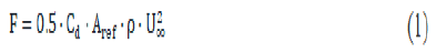
Where ρ is the density of the fluid and Aref is the reference area. In this case, it is an area of a circle with the same diameter as the ref analyzed sphere. U∞ is the velocity of the mean flow while Cd is the drag coefficient (Figure 2).
Drag coefficient of the ball formatting and inserting equations
The drag coefficient (Cd), of the ball (sphere), is depending on the Reynolds number (Figure 3) which is calculated as:

Figure 3: Standard plot of coefficient of drag versus Reynolds number for spherical bodies.
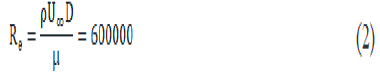
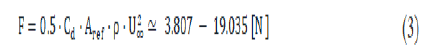
The estimation of the ball drag coefficient is not straightforward. Considering the Reynolds number of 600000, according to NASA documentation, the drag coefficient (Cd) can be estimated in a range from (0.1-0.5), which leads to evaluating the drag force acting on the ball to:
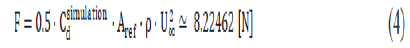
The CFD simulation, described below, gives the drag coefficient Cd=0.215 which leads to the drag force:
Beam deformation and stress analytical solution
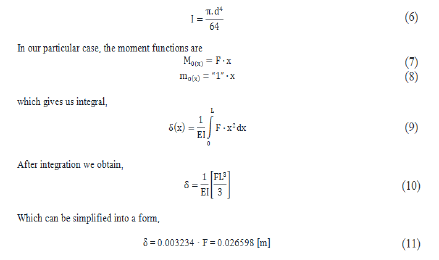
Deformation analysis: Let’s consider a simplified one-dimensional model of a cantilever beam, with one fixed end and one free end (Figure 4) [3]. Let the beam length be L and the beam is loaded with a single point load (force F) at its end. We can obtain an analytical solution of beam displacement, δ(x) anywhere along the beam by applying Mohr integral formula:

Figure 4: Cantilever beam sketch: Deformation analysis.
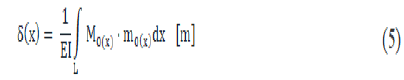
Where, M0(x) denotes bending moment function, along the beam length (x-coordinate, x=0 at the free end and x=L at the wall), from the load by the force F. The m0 (x) means bending moment, along the beam length (xcoordinate, x=0 at the free end and x=L at the wall) from unit dimensionless force (“1”) applied at the very point, where we want to analyze displacement. E is the Young’s Modulus of Elasticity of the beam material and I represent the Moment of Inertia of a beam cross-section. For circular beams, “I” by expressed as:
Stress analysis: Let’s consider the same cantilever beam, with one fixed end and one free end. Let the beam length be L and the beam is loaded with a single point load (force F) at its end (Figure 5).

Figure 5: Cantilever beam sketch: Stress analysis.
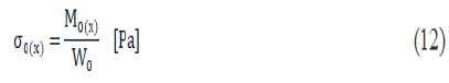
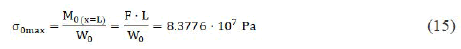
where σ0(x) is the Stress Function, along the beam length (x-coordinate, x=0 at the free end and x=L at the wall), from the load by the force F (Table 1). denotes bending moment function, along the beam length (x-coordinate, x=0 at the free end and x=L at the wall), from load by the force F. Wo declares resistant moment of the neutral axis of bending, which is moment of Inertia divided by the longest distance of thread from the neutral axis, in our case of circular beam it is:
| Mesh elements | Points | Faces | Internal faces | Faces per cell | Hexahedra |
|---|---|---|---|---|---|
| # | 535722 | 1512960 | 1487592 | 6.128328 | 458023 |
| Mesh elements | Prisms | Pyramids | Tet wedges | Polyhedra | Cells |
| # | 1056 | 0 | 0 | 30541 | 489620 |
Table 1: FEA meshing: Values for different parameters

In the structural analysis, we are typically interested in the maximal value of the stress. That can be found by the derivation of stress or moment function to find maximal or minimal values
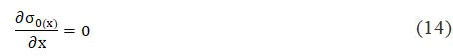
In our model, we can simply assume, that the stress function is linear and the maximal stress will be at the wall (x=L), so
Beam-ball full case simulation in TCAE
The beam-ball surface model is created in CAD and loaded in TCAE in the form of fine 3D STL surface files. All the simulation setup is done in the TCAE graphical interface. The TCAE simulation workflow is completely automated. If the simulation setup is completed, the whole simulation process is run with a single click of the Run all button in GUI, or s single command is executed in the command line.
TCAE consists of different software modules [5]. The simulation workflow chronological order is following: Start → CFD mesh → FEA mesh → CFD simulation → FSI → FEA simulation → Report. This particular case uses the following TCAE software modules: The TMESH module creates meshes both for CFD and FEA and makes them ready for the simulation. TCFD module runs CFD simulation and writes down the CFD results report. TFEA module makes FSI conversion, runs FEA simulation, and writes down the FEA results report.
The aerodynamic effects acting on the beam itself are neglected. The aerodynamic simulation is performed only around the ball (sphere) to benefit from a completely symmetrical mesh to receive as accurate results as possible. Note, the simulation results will be compared with an analytical solution, which also considers the point load at the end of the beam.
CFD mesh
The computational mesh for CFD was produced using the snappyHexMesh open-source application in an automated software module called TMESH. A cartesian block mesh was constructed as an initial backdrop mesh for each model component (in this case, just one component-Virtual Tunnel), which was refined together with the simulated item (Figure 6). The virtual tunnel is 20 meters long, 8 meters tall, and 8 meters broad. A cube with a 200 mm edge is the most basic mesh cell size. Three more refining regions have been added. The mesh is fine-tuned until it reaches the model wall. To better handle mesh size, the mesh refinement levels can be simply modified to achieve a coarser or finer mesh. Layers of inflation can be easily managed. In this particular case, there are 5 inflation layers with an expansion ratio of 1.20. The final CFD mesh used for the simulation has in total 489,620 cells and consists mostly of hexahedrons. SnappyHexMesh, a meshing application, is not a mandatory meshing tool for TMESH (Figure 7). Any other external mesh in MSH, CGNS, or OpenFOAM format can be loaded straight into TMESH if necessary (Table 1).

Figure 6: Rendered view of the ball (sphere).

Figure 7: a) Virtual tunnel; b) CFD meshing of ball as well as around the ball.
FEA mesh
The computational mesh for CFD was produced using the NetGen opensource tool and an automated software module called TMESH (Figure 8).

Figure 8: a) Parameters for meshing; b) FEA meshing of the ball.
Setup
CFD simulation case setup: The TCAE software module TCFD is used to oversee the CFD simulation. GUI in Paraview is used to set up and run the numerical simulation. The OpenFOAM open source application is used by TCFD.
It is a virtual tunnel-type simulation with a steady state and incompressible physical model. The RANS k-ω SST turbulence method is used with a turbulence intensity of 1%. Wall surface roughness is neglected but the wall functions are chosen for the wall treatment. The number of components, speed lines, and simulation points is taken as 1. Air is the primary fluid with a dynamic viscosity of 1.8 × 10⁻⁵ Pa-s and a standard density of 1.225 kg m-3. The inlet velocity is 30 ms-1 and the outlet pressure is zero (i.e. the gauge pressure).
FEA simulation case setup
The TCAE software module TFEA is used to maintain the second-order Finite Element Analysis (FEA) simulation. The TFEA GUI in para view is used to build and run the FEA simulation. Calculix open-source applications are often used by TFEA. The isotropic structured material is chosen for the simulation is steel with a density of 7800 kg m-3, Young’s modulus, and Poisson ratios are 2.1 × 10¹¹ Pa and 0.3 respectively.
Simulation setup
The simulation was run in a steady-state condition in the autonomous TCAE workflow for a flow velocity of 30 m/s. TCFD can write down the results at any point during the simulation. Figure 9 shows how the convergence of any parameter is tracked during the experiment.

Figure 9: Simulation setup: Residual versus iteration plot.
Results and Discussion
The compared results differ by about 5% in maximal deformation and 10% in maximal stress which meets well the original expectation (Table 2). Despite the analytical 1D solution can be assumed as final, the simulation results can slightly differ according to the simulation settings. Especially, the CFD mesh and FEA mesh density may have certain effects on the simulation results. The following figures show the deformed beam stress magnitude and displacement magnitude. The deformation on this ten times larger for a better visual perception (Figure 10).
| Analytical solution | TCAE simulation | |
|---|---|---|
| Max deformation (mm) | 26.6 | 27.75 |
| Max stress (MPa) | 83.78 | 92.48 |
Table 2: The final comparison of the analytical solution with the simulation results.

Figure 10:a) Stress magnitude and b) displacement magnitude.
Conclusion
• The complex FSI analysis was performed successfully. It has been
shown that the 3D TCAE simulation prediction gives a good agreement
with the 1-D analytical solution.
• TCAE showed to be a very effective tool for CFD, FEA, and FSI
engineering simulations.
• This study will further help aerodynamic experts, wind engineers, and
structural designers to easily and efficiently use the process designed by
authors for their respective applications.
Acknowledgement
The research has been duly facilitated by the dpartment of mechanical and civil engineering graphic era deemed to be university and state key laboratory of disaster prevention in civil engineering, Tongji University, China for funding the research study.
Author Contribution
All authors contributed equally to the research and writing. All authors have read and agreed to the published version of the manuscript.
Funding
No external funding has been provided.
Conflicts of Interest
The authors declare no conflict of interest.
References
- Anwer M. Fluid-structure interaction. Handbook of Machinery Dynamics, 1st edition, CRC Press, 2000, pp. 195-354.
- Jian W. Propagation of a Gaussian-Schell beam through turbulent media. J Mod Opt. 1990;37(4):671-84. [Crossref][Googlescholar]
- Wu J, Boardman AD. Coherence length of a Gaussian-Schell beam and atmospheric turbulence. J Mod Opt. 1991;38(7):1355-63. [Crossref][Googlescholar]
- Achilles D, Silberhorn C, Sliwa C, et al. Photon-number-resolving detection using time-multiplexing. J Mod Opt. 2004;51(9-10):1499-515. [Crossref][Googlescholar]
- Stefanov A, Gisin N, Guinnard O, et al. Optical quantum random numbesr generator. J Mod Opt. 2000;47(4):595-8. [Crossref][Googlescholar]
- Anand V, Christov IC. Steady low Reynolds number flow of a generalized Newtonian fluid through a slender elastic tube. ArXiv preprint. 2018;62-72.
- Maalini PM, Prabhakar G, Selvaperumal S. Modeling and control of ball and beam system using PID controller. In2016 International Conference on Advanced Communication Control and Computing Technologies (ICACCCT). 2016;322-326. [Crossref][Googlescholar]
- Buza G, Milton J, Bencsik L, Insperger T. Establishing metrics and control laws for the learning process: ball and beam balancing. Biolo Cybernetics. 2020;114(1):83-93. [Googlescholar]
- Ali AT, Ahmed AM, Almahdi HA, et al. Design and implementation of ball and beam system using PID controller. MAYFEB J Electr Comput Eng. 2017;11;1. [Googlescholar]