Complex Evolution Dynamics of Insect Population

Received: 18-Feb-2021 Accepted Date: Mar 01, 2021; Published: 09-Mar-2021, DOI: 10.37532/2752-8081.21.5.25

Citation: Lal Mohan S, Nandlal Mandal. Complex Evolution Dynamics of Insect Population. J Pur Appl Math. 2021; 5(2):16:22.

This open-access article is distributed under the terms of the Creative Commons Attribution Non-Commercial License (CC BY-NC) (http://creativecommons.org/licenses/by-nc/4.0/), which permits reuse, distribution and reproduction of the article, provided that the original work is properly cited and the reuse is restricted to noncommercial purposes. For commercial reuse, contact reprints@pulsus.com

Abstract

Principles of nonlinear dynamics applied to investigate complex evolution of insect population. LPA model considered in this regard and studies carried out to visualize regular and chaotic evolutions.

Different sets of bifurcation diagrams obtained by varying death rate parameter μa of adult population and that of μl , the larvae population. Regular and chaotic attractors obtained for different sets of values of parameters.

Numerical calculations carried out to obtain Lyapunov exponents for identification of regular and chaotic evolution and to obtain topological entropies, which provide presence of complexity in the system.

Calculations further extended to obtain the correlation dimension of a chaotic attractor.

Keywords

Chaos, Lyapunov Exponents, Bifurcation, Topological Entropy

Introduction

Emergence of the concept of chaos and complexities in many real systems encouraged researchers to take active interest in applications of deterministic principle and to take active interest in studying dynamics of evolutions of plants, insects and animals. Regular and chaotic evolutionary behavior in nonlinear systems has fascinated scientists of recent times and exciting results discovered. The biological systems are complex and multicomponent, [1-4]. Such systems spatially structured and their individual elements possess individual properties. A sincere study on these systems provides results to understand how the deterministic rules capable to explain the complex fluctuations in living systems.

Due to non-linear nature, most real systems exhibit chaos and complexity character during evolution. Complexity can viewed as its systematic nonlinear properties and it is due to the interaction among multiple agents within the system. Presence of complexity in a systems havefeatureslikecoexistenceofm ultipleattractors,bistability,intermittency,fractalproperty,cascading failures, often exhibit hysteresis, network of multiplicity, emergent phenomena and some more properties, [5-8]. The measure of complexity is provided by topological entropy, more topological entropy in a system signifies the system is more complex, [9-12]. These articles have also explained complexity of different types observed in real systems. Lyapunov exponents,(LCEs), stand for measure of chaos; it provides indications of regular and chaotic evolution. Positive (LCEs) signifies the presence of chaos and its negative value stands for regularity in the system, [13-17].

Insect evolution is metamorphosis since a series of big changes occurring during growth and development of insects. Their evolution passes through four distinct stages: egg, larva, pupa and adult [18-22]. Among insects going through such stages can be listed as butterflies, moths, beetles, flies, bees, wasps, and ants. While transforming from one stage to another stage an insect has to molt its skin and each time it emerge larger and of different form until it reaches the adult stage. Most insects have annual non-overlapping generations.

Adults may lay eggs in spring or summer, and then die. The eggs hatch out into larvae, which eat and grow in a pupal stage. The adults emerge from pupae. Some recent investigations designed to study evolutionary changes in insect populations like flour beetle Tribolium, in LPA model. Considering the discreteness of individuals and for demographics to chasticity, modified deterministic discrete states as well as stochastic discrete state in LPA models, studies carried out and a number of exciting results are drawn.

While studying evolution of insects in the LPA model, it seems reasonable to observe bifurcation and other properties by varying also the mortality rate μ₁, of the larvae population in addition to that of μ_a the adult population. Then, non-consideration of mortality rate μ_p or assumption that μ_p= 0, for pupa population, may not match with real situation. This rate μ_p may possibly be small but not zero. Presence of complexity and existence of regularity and chaos during evolution require investigation in different parameter space.

The objective of this investigation is further exploration of the evolutionary properties of LPA system for insect population. Study would include visualization of regular and chaotic evolution through bifurcation diagrams by varying, in turn, μ₁ and μ_a while keeping other parameters constant and, assumption of cases μ_p = 0 as well as μ_p< 0. Proper numerical simulations carried out to calculate and draw the regular and chaotic attractors for different sets of parameters of the system. Calculations further extended to obtain quantities like Lyapunov exponents, which confirm presence of regularity and chaos; topological entropies, which provide presence of complexity in the system and correlation dimension, which provides the dimensionality of a chaotic attractor.

The Mathematical Model

Discrete formulation of LPA for evolution of insect populations followed by equations, [2,3],

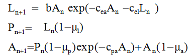          (1)

In (1), Ln, Pn, stand, respectively, for larva, pupa and adult populations at the n^th generation. The parameter b stands for the birth rate of the species, (the number of new larvae per adult each unit time), and μ₁, μ_p, μ_a stand for the death rates of larva, pupa and adult, respectively. The fractions exp(−Cea An) and exp(−Cel Ln), respectively, are the probabilities that an egg is not eaten in the presence of adults An and larvae Ln. Also, the fraction exp(− Cpa An) stands for the survival probability of pupa in presence of adults An. The parameters, C_ea, C_el, C_pa assigned as cannibalism coefficients, [4].

Bifurcation Phenomena and Attractors

Bifurcations in a system show the changes occurring in the qualitatives tructure of the system during evolution when a particular parameter of it varies while other parameters kept constant.

Below Figure, Figure 1, show bifurcations scenario of system (1) when 0≤μa≤1.0, a various parameter space of parameters Cea, Cel, Cpa, b, μ l, and μ_p.

Figure 1a) Bifurcation diagrams when C_ea=0.009, C_el=0.012, C_pa=0.012, C_pa=0.004, b =7.48, μ_l=0.267, μ_p =0.1, and for 0 ≤μ_a≤ 1.0

Figure 1b) Bifurcation diagrams when C_ea=0.011 C_el=0.012, C_pa=0.004, b =11.68, μ_l=0.513, μ_p =0.001 And for 0≤ μ_a≤1.0.

Figure 1c) Bifurcation diagrams when C_ea=0.011, C_el=0.012, C_pa=0.02, b =11.68, μ_l=0.213, μ_p =0.001, and for 0≤μ_a≤1.0.

Figure 1d) Bifurcation diagrams when C_ea=0.011, C_el=0.012, C_pa=0.017, b =11.68, μ_l=0.213,μ_p =0.0, and for 0≤μ_a≤1.0.

Figure 1e) Bifurcation diagrams when C_ea=0.011, C_el=0.012, C_pa=0.017, b=11.68, μ_l=0.213, μ_p =0.0, and for 0.8≤μ_a≤1.

The cannibalism coefficient Cpa play an active role in deciding regular and chaotic evolution of the system. Varying μl, 0 ≤ μl ≤ 1.0, a complete regular and chaotic case of bifurcation are observed for different sets of values of other parameters as shown in Figure 2. Regularity indicates the possible coexistence. In this range of μl, interesting cases of chaos observed for three different μa, shown in Figure 3.

Figure 2a) Bifurcation diagrams when C_ea=0.009, C_el=0.012, C_pa=0.004, b =5.55, μ_a =0.19 μ_p =0.1, and for 0≤μ_l≤ 1.

Figure 2b) Bifurcation diagrams when C_ea=0.01, C_el=0.03, C_pa=0.009, b =8.5, μ_a =0.9, μ_p =0.01, and for 0≤μ_l≤ 1.0.

Figure 3) Bifurcation diagrams when0≤μ_l≤1.0 and for values of C_ea= 0.015, C_el= 0.0115, C_pa =0.016, b =6.5, μ_p=0.01 and with cases (a)μ_a=0.87, (b)μ_a=0.875, (c) μ_a=0.88.

Formation of Chaotic Attractors

System (1) displays chaotic evolution in some parameter space. In the following Figures Figure 4, time series curves and phase plots shown for such chaotic evolution. A chaotic attractor for the motion and is shown in Figure 5.

Figure 4a) Chaotic times series and phase attractors of LPA system (1) for values of C_ea=0.009, C_el=0.012, C_pa=0.004, b =7.48, μ_l=0.267, μ_a =0.98, μ_p=0.01.

Figure 4b) Chaotic time series and phase attractors of LPA system (1) for values of C_ea=0.011, C_el=0.012, C_pa=0.02, μ_l=0.213, μ_a=0.8, μ_p=0.001, b=11.68.

Figure 5) A chaotic attractor in (L, P) plane when C_ea=0.009, C_el=0.012, C_pa=0.004, b=7.48, μ_l = 0.267, μ_a =0.98, μ_p=0.01.

Plots of Lyapunov Exponents and Topological Entropies

(a) Lyapunov Exponents(LCE): Lyapunov exponents are perfect measures of regular and chaotic motion. LCEs are positive for chaotic evolution and negative for regular motion.

Higher and lower positive LCE values indicate, respectively, strongly and weakly chaotic evolutions, [19-22].

The Plots of Lyapunov exponents for regular and chaotic evolutions of system (1) for different parameters spaces presented in the sets of Figure, Figure 6.

Figure in Figure 6a are for regular and chaotic motion with two different μ_a, (0.4, 0.95), with same values of other parameters.

Plots in Figure 6b are drawn for three different sets of values of (μ₁,) when b, Cea, Cel and Cpa are kept constant; plots in Figure 6c are for different values of Cel while other parameters are same; plots in Figure 6d are to show the influence of cannibalism coefficients Cea, Cel and Cpa. The last plots Figure 6e, correspond to the bifurcation Figure 3a μ_a= 0.87 and (b) μ_a = 0.88.

Figure 6a) LCEs plots for values of parameters cea=0.009, c_el=0.012, c_pa=0.004, b=7.48, μ_a=0.267, μ_p=0.1 and then in plot (a) μ_a=0.4, in plot (b) μ_a=0.95.

Figure 6b) LCEs plots for cea=0.011,c_el= 0.012, c_pa= 0.017, b=11.68 and, in(a) μ_l=0.513, μ_p= 0.001 and μ_a= 0.5;in (b) μ_l=0.513, μ_p=0.001 and μ_a=0.8; in plot (c) μ_l=0.213, μ_p=0.0 and μ_a=0.18.

Figure 6c) Plots of LCEs for parameters b=8.5, μ_l=0.4, μ_p=0.01, μ_a=0.9, C_ea=0.02, C_pa= 0 .012 and, in (a) C_el=0.04; in (b) C_el=0.045; in (c) C_el=0.05.

Figure 6d) LCEs plots for values b=11.5, μ_l=0.5, μ_p=0.01, μ_a= 0.8, and in (a) C_el= 0.02 and C_pa=0.004; in (b) C_ea=0.02and C_pa=0.004; in (c) C_ea=0.02 and C_el=0.04.

Figure 6e) Plots of LCEs for parameters cea=0.015,c_el= 0.015, c_pa= 0.016, b= 6.5, μ_p=0.01, μ_l=0.35; (a) μ_a=0.87 and (b) μ_a= 0.88.

(b)Topological Entries: Topological entropy is an invariant of topological conjugacy and an analogue of measure theoretic entropy. It provides a numerical measure for the complexity of an endomorphism of a compact topological space, [5]. A complex system can viewed as that composed on many components, which may interact with each other. During evolution, in addition to chaos, the system may show some degree of spontaneous order, numerosity and robustness. Complexity in the system measured topological entropy, which is a non-negative number. More increase in topological entropy of a system means it is more complex. Actually, it measures the exponential growth rate of the number of distinguishable orbits as time advances. Topological entropy calculated statistically in the following way:

Consider a finite partition of a state space X denoted by P = {P1, P2, P3, PN}. Then a measure μ on X with total measure μ(X) = 1 defines the probability of a given reading as p_i = μ (P_i ) , i = 1, 2, . . , N.

Then the entropy of the partition be given by

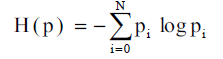           (3)

The topological entropy, H ( p ) is a positive quantity and more topological entropy of a system signifies it is more complex.

As it appears from plots Figure 7, case (a), when Cea=0.009, Cel=0.012, Cpa=0.004, b=7.48, μ_p=0.1 and μ₁=0.267, there is no increase of entropy for 0 ≤ μ_a ≤ 1.0. Significant increase in topological entropies occur in cases (b) and (c) for variation of μ₁. These cases describe the complex nature of evolution in the system in these parameter spaces

Figure 7) Topological entropy plots for parameters: (a) C_ea=0.009, c_el=0.012, c_pa= 0.004, b=7.48, μ_p= 0.1, μ_l=0.267 (b) C_e= 0.01, c_el=0.03, c_pa=0.009, b=8.5, μ_p=0.001, μ_a=0.9, (c) C_ea=0.02.

(C) Correlation Dimension: Correlation dimension provides the measure of dimensionality of the chaotic attractor. This is calculated statistically with the application of Heaviside function. Using the steps of Mathematica suggested in, first data for correlation integral C(r) calculated for certain r. Then, plotted the curve log C(r) / log r against r shown in Figure 8.

Figure 8) Plot of correlation integral data; when C_ea=0.009, C_el=0.012, C_pa=0.004, b =7.48, μ_l=0.267,μ_a=0.98,μ_p=0.01.

After this, we have applied a linear fit criterion to the correlation data and obtained the equation of the straight line

y = 2.77931 x + 0.692407           (2)

The y-intercept of this straight line is 0.692407 and so, [18], the correlation dimension of the chaotic attractor Figure 2a is, approximately, D_c ≅ 0.692. Following this procedure, one can obtain correlation dimension for any other attractor.

DISCUSSION

Different sets of bifurcation diagrams obtained by varying death rate parameter μa of adult population and that of μl, the larvae population, (Figure 1 – Figure 3). As in a variety of nonlinear systems, one observes appearance of periodic windows within chaotic region during bifurcations of the system shown in Figure 1 and in Figure 2. Such periodic windows become gradually shorter and appearances become more frequent while moving forward in parameter space. This signifies an intermittency character. Bifurcation diagrams shown in Figure 3, are of strange type; it may be because of overlapping of values. The LCEs plots for such cases shown in Figure 6(e).

Regular as well as chaotic evolution observed for different sets of parameter values and measured by LCEs shown through Figure 6(a) – 6(e). Here, Figure 6(b) shows the influence of parameters μl, μ_p and μa for regular and chaotic motions. Figure, Figure 6(c) and Figure 6(d) are drawn to show the role of cannibalism coefficients cea, cel, cpa in changing the dynamic evolution of system (1). One notice that in the parameter space shown in Figure 6(d), for 0.005 ≤ cea≤ 0.02, the regular motion changes to chaos and then, again, return to regularity. Similar is the case for 0.02 ≤ cel≤ 0.031. But cpa at a value 0.01 show regularity and then with increasing its value evolution becomes chaotic.

Presence of complexity in the system implies significant increase in topological entropy. From the plots of topological entropies, Figure 7, one observes: in plot (a) nil increase of topological entropy; in plot (b) topological entropy increases significantly in 0.9 ≤ μl ≤ 1.15; in plot (c) fluctuating type of its increase in 0.8≤ μl ≤ 0.95 and the increase in 1.0 ≤ μl ≤ 1.2; in plot (d) significant increase of topological entropy in 0.875 ≤ μl ≤ 1.15. Similar results can be obtained by varying other parameters, (e. g. μa, μ_p). It has also been observed that even if the system is regular complexity may exists and, also, during a chaotic evolution complexity may or may not be exhibited. Correlation dimension of the chaotic attractor shown in Figure 5, is obtained through data of plot, Figure 8, as D_c≅0.692.

REFERENCES

1. May RN. Simple mathematical models with very complicated dynamics. Nature. 1976;261:459-467.
2. Rial JA. Chaos: An Introduction to Dynamical Systems. American Scientist. 1997; 85:487.
3. Dennis B. Estimating chaos and complex dynamics in an insect population. Ecological Monographs. 2001; 71:277-303.
4. King AA. Anatomy of a chaotic attractor: subtle model-predicted patterns revealed in population data. Proceedings of the National Academy of Sciences. 2004; 101:408-13.
5. Adler. Topologicalentropy. Trans Amer Math Soc.1965;114:309-319.
6. Balm forth NJ. Topological entropy of one-dimensional maps: Approximations and bounds. Physical review letters. 1994;72(1):80.
7. Bowen R. Topological entropy for noncompact sets. Transactions of the American Mathematical Society. 1973;184:125-36.
8. Baldwin SL, Slaminka EE. Calculating topological entropy.  J Statistical Physics. 1997; 89:1017-33.
9. Beddington JR. Dynamic complexity in predator-prey models framed in difference equations. Nature. 1975;255:58-60.
10. Xiao Y. Dynamic complexities in predator–prey ecosystem models with age-structure for predator. Chaos, Solitons & Fractals. 2002; 14:1403-1411.
11. Saha LM. On Nonlinear Dynamics, Chaos and Complexities. IJIAM. 2016; 7:270-84.
12. Kaitala V, Heino M. Complex non-unique dynamics in simple ecological interactions. Proceedings of the Royal Society of London. Series B: Biological Sciences. 1996; 26:1011-5.
13. Benettin G. Lyapunov characteristic exponents for smooth dynamical systems and for Hamiltonian systems; a method for computing all of them. Part 1: Theory. Meccanica. 1980; 15:9-20.
14. Abarbanel HD. Local Lyapunov exponents computed from observed data. J Non Sci. 1992; 2:343-365.
15. Grassberger P, Procaccia I. Measuring the strangeness of strange attractors. In The Theory of Chaotic Attractors 2004. Springer, New York, NY.
16. Saha LM, Kumra N. On dynamics of chaotic evolution in food chain model. J Math Comput Sci. 2013; 3:823-840.
17. Erjaee GH, Alnasr M. Phase synchronization in coupled Sprott chaotic systems presented by fractional differential equations. Discrete Dynamics in Nature and Society. 2009 .
18. Britton N. Essential mathematical biology. Springer Science & Business Media. 2005.
19. Costantino RF. experimentally induced transitions in the dynamic behaviour of insect populations. Nature. 1995; 375:227-30.
20. Cushing JM. The LPA model. Fields Institute Communications. 2004; 43:29-55.
21. Nagashima H. Introduction to chaos: physics and mathematics of chaotic phenomena. CRC Press; 2019.
22. Martelli M. Introduction to discrete dynamical systems and chaos. John Wiley & Sons; 2011.