
Evaluation of integrated hydro geosphere hydrologic model in modeling of large basins subject to severe withdrawal
2 Department of Water Engineering and Hydraulic Structures, Faculty of Civil Engineering, Iran
3 Water Engineering Department, College of Agriculture, Bu-Ali Sina University, Hamadan, Iran
4 Department of Civil Engineering, Isfahan (Khorasgan) Branch, Islamic Azad University, Isfahan, Iran, Email: koa.askari@khuisf.ac.ir
5 Department of Biological and Agricultural Engineering and Zachry Department of Civil Engineering, Texas A and M University, 321 Scoates Hall, 2117 TAMU, College Station, Texas, USA
Received: 26-Dec-2017 Accepted Date: Jan 01, 2018; Published: 25-Jan-2018
Citation: Talebmorad H, Eslamian S, Abedi-Koupai J, et al. Evaluation of integrated hydro geosphere hydrologic model in modeling of large basins subject to severe withdrawal. J Environ Chem Toxicol. 2018;2(2):30-40.
This open-access article is distributed under the terms of the Creative Commons Attribution Non-Commercial License (CC BY-NC) (http://creativecommons.org/licenses/by-nc/4.0/), which permits reuse, distribution and reproduction of the article, provided that the original work is properly cited and the reuse is restricted to noncommercial purposes. For commercial reuse, contact reprints@pulsus.com
Abstract
Simulation of large basins (over 1,000 km2) is needed for largescale water resources planning and management. Due to increased volume of calculations and increased heterogeneity, basin simulation is challenging. In areas with severe withdrawal of water resources, simulating and having the ability to predict future changes is important, while severe withdrawals complicate issues and simulation. The aim of this study is to evaluate the ability of Hydro Geosphere, a fully integrated hydrologic model, to simulate a large basin (Hamadan-Bahar Catchment, Iran) with an area of 2,456 km2 and severe groundwater withdrawals. In this study, fully-integrated surface/ subsurface flow modeling was done using the Hydro Geosphere model. Simultaneous solution of surface and groundwater flow equations and calculation of actual evapotranspiration as a function of soil moisture in each unit of evaporation zone improves the simulation of interdependent processes such as aquifer recharge and drainage, which is one of the difficult issues in modeling. To obtain initial conditions, the model was used in steady state mode using 20-year average of rainfall data and withdrawal from the aquifer. Then, to apply the model in unsteady state and evaluate its performance in daily stresses, the model was used for the period of 19922005 and parameters were calibrated. Validation was done for the period of 2006-2010 and results showed satisfactory hydrologic simulation of the study area.
Keywords
Hydro geosphere; Integrated hydrologic modeling; Surface watergroundwater interaction; Groundwater withdrawal; Hamadan-Bahar basin; Evaporation
Effective management of watersheds and ecosystems requires understanding of hydrological processes. Increasing use of models has enhanced the ability to assess and predict catchment behavior. In these models, complex hydrologic conditions and transmission processes are usually simplified. Due to the multiplicity of factors affecting the catchment behavior is usually simulated using, numerical models. Many numerical models have been developed with varying degree of complexity. Numerical models are based on numerical methods which are used for solving problems on computers by numerical calculations, often giving a table of numbers and/or graphical representations or figures. Numerical methods tend to emphasize the implementation of algorithms. The aim of numerical methods is therefore to provide systematic methods for solving problems in a numerical form. The process of solving problems generally involves starting from an initial condition, using high precision digital computers, following the steps in the algorithms, and finally obtaining the results [1]. Numerical methods are becoming more and more important in mathematical and engineering applications not only because of the difficulties encountered in finding exact analytical solutions, but also because of the ease with which numerical techniques can be used in conjunction with modern high-speed digital computers [2]. In many situations, information about the physical phenomena like hydrologic cycle involved is always pervaded with uncertainty. The uncertainty can arise in more than one place such as experiment part, data collection, measurement process as well as when determining the initial values [3]. Therefore, it is necessary to consider the accuracy of input data and uncertainty in the results.
A proper model for basin simulation should be selected, depending on the purpose of modeling, conditions of the area, and the available data. The aim of this study was to assess the capability of a comprehensive hydrologic model of Hydro Geosphere i(HGS) n simulating a large catchment (Hamadan-Bahar) with an area of 2456 km2 that is being subjected to severe groundwater withdrawal. Sudicky et al. [4] employed the model integrating surface and subsurface flow in area of 17 km2 in southern Ontario, Canada. The capability of the HGS model with integrated surface and subsurface flow and the effect of rainfall time series, which included the average annual, average monthly and average daily values, were assessed for the simulation of average flow from the river to the aquifer and vice versa near the main drainage channel. They found that the model was not able to simulate the maximum flow between river and aquifer with monthly or annual rainfall time series [5]. Jones et al. [6] evaluated the HGS model in the Grand River basin (area of 75 km2 area) in southern Ontario and good agreement between simulated and observed groundwater pattern, confirming the efficiency of the Richards equation in the unsaturated zone [7].
Cornelissen et al. [8] assessed the influence of spatial resolution on the simulation of spatio-temporal soil moisture variability using Hydro Geosphere in a forested catchment (area of 0.27 km2). Discharge and soil moisture simulations were in an agreement with measured water balance and discharge dynamics.
Cornelissen et al. [9] investigated the parameter sensitivity in HGS in the Erkensruhr catchment (area of 41.9 km2) and precipitation was reported as most sensitive input data with respect to total runoff and peak flow rates, while simulated evapotranspiration patterns were reported as most sensitive to spatially distributed land use parameterization
Materials and Methods
Description of the study area
The Hamadan–Bahar basin with an area of 2456 km2 is situated between longitudes of 48° 7’ E and 48° 52’ E and latitudes of 34°35’N and 35°12’N in western Iran (Figure 1). In this basin, most of the rivers originate from southern heights (Alvand Mountains). The outlet of basin is Koshkabad in the north-east. The mean elevation of the watershed is 2038 m above mean sea level. The average daily discharge at Koshkabad station was 2.5 m3 s−1 for the period of 1992–2008, with a minimum value of zero and a maximum value of 90.4 m3 s−1. The climate of the region is semiarid with mean annual precipitation of 324.5 mm and mean annual temperature of 11.3°C. In the Hamadan–Bahar basin, groundwater is the only available and widely used source of drinking water for rural and urban communities and also for irrigation. Groundwater supplies approximately 88% of the water consumed in the Hamadan. The area of the main aquifer of the plain is 468 km2 and geologically, Hamadan–Bahar aquifer is located in the Sanandaj- Sirjan metamorphic zone (Hamadan Regional Water Authority, HRWA). The alluvial aquifers consist mainly of gravel, sand, silt and clay [10].

Figure 1: Study area of Hamadan-Bahar watershed in Hamadan province, Iran
Model description
Hydro Geosphere conceptualizes the hydrologic system comprising surface and subsurface flow regimes with interactions [11]. The model takes into account all key components of the hydrologic cycle. For each time step, the model solves surface and subsurface flow and mass transport equations simultaneously and provides complete water balance and solute budget. The surface water budget can be written as:

Giving the total hydrologic budget as the sum of Equations 1 and 2:
where P is the net precipitation (actual precipitation - interception), QS1 and QS2 are the surface water inflow and outflow, QGS is the surface/subsurface water interactive flow, I is the net infiltration, ETS is the evapotranspiration from the surface flow system, QWS is the overland water withdrawal, ΔSS is the surface water storage over time step Δt, QG1 and QG2 are the subsurface water inflow and outflow, ETG is the evapotranspiration from the subsurface flow system, QWG is the subsurface water withdrawal and ΔSG is the subsurface water storage over time step Δt.
For integrated analysis, Hydro Geosphere utilizes mass conservation modeling that fully couples surface flow and solute transport equations with the 3-D, variably-saturated subsurface flow and solute transport equations. Both surface and subsurface modeling codes are robustly linked. The model is a powerful numerical simulator specifically developed for supporting water resources and engineering projects pertaining to hydrologic systems with surface and subsurface flow and mass transport components [12].
Conceptual model
Hydro Geosphere can only use two-dimensional grid files produced with grid builder or GMS software for 3D grid computing. Because of the high abilities of GMS, this model was used to create the layers of conceptual model [13]. According to the available geological maps of the area, exploration and observation well data in the basin and measured data, there is only one free aquifer in the region. The first step in creating the conceptual model is to define the surface and bottom layers of the aquifer. The top and bottom layers of nodes represent the soil surface and the bedrock, respectively. Elevations of the surface nodes are calculated using the basin DEM (Digital Elevation Model), whose pixels have dimensions equal to 20 20 m, and the bedrock node elevations are calculated using contour map provided in basin geological report. Due to hardware limitations and the vastness of basin the horizontal grid dimension equal to 1000 1000 m was chosen and then for increasing the accuracy of modeling the withdrawal wells were added to the mesh as nodes. There were 825 withdrawal wells in the plain. Finally, the surface layer was characterized with 3495 nodes and 6757 elements (Figure 2).

Figure 2: Horizontal grid generated using GMS
On vertical grid, the region was divided into two upper (0-5-meter depth) and lower (more than 5-meter depth) parts. In order to increase the accuracy in evapotranspiration calculation, the upper part was divided into six layers with an interval of 1 meter and the lower part was divided at an interval of 10 meters [14]. Thus, the whole basin was divided into 14 layers. Due to the reduction in thickness, the distance between the layers was reduced in the adjacent and non-aquifer areas. To avoid interference and zero thickness of the layers, the minimum distance of the vertical networks was set at 0.2 m. Finally, a three-dimensional mesh, composed of several layers of 6-node triangular prismatic elements, was generated (Figure 3).

Figure 3: Spatial discretization of basin generated by HGS (Elevation exaggeration is 10)
After mesh generation the properties of each domain are entered and hydrologic parameters required for the fully-coupled simulation are listed, as in Table 1, along with their domain of application [14]. Maps of land use, soil texture, hydraulic conductivity, and specific yield values were obtained from the drawings and specifications required and previous studies in this area were extracted and entered into the model (Figures 4-6).
| Domain | Parameters | Abbreviation | Dimension |
|---|---|---|---|
| Subsurface | Full saturated hydraulic conductivity | K | [LT-1] |
| n Total porosity [–] | n | [-] | |
| Specific storage | Ss | [L-1] | |
| Van Genuchten parameter | α | [-] | |
| Van Genuchten parameter | β | [L-1] | |
| Residual water saturation | Swr | [-] | |
| Surface | Manning roughness coefficient | nx | [L-1/3T] |
| Manning roughness coefficient | ny | [L-1/3T] | |
| Evapotranspiration | Evaporation depth | Le | [L] |
| Leaf Area Index | LAI | [-] | |
| Root depth | Lr | [L] | |
| Transpiration fitting parameters | C1, C2, C3 | [-] |
Table 1: List of hydrologic parameters used in flow model

Figure 4: Land use, vegetation coverage and hydraulic conductivity map of the plane

Figure 5: Withdrawal wells location

Figure 6: Bedrock map of aquifer
Boundary conditions
Since the study area from all sides, except the basin outlet, is limited to impermeable mountains, no flow boundary conditions were considered for the surrounding area and the bed rock of the basin. In addition, daily rainfall and potential evapotranspiration, of which are kind of flux boundary condition, were considered as specified rainfall and specified evaporation in the model. In the outlet part of the basin, because of the hydraulic connection with the Kabudrahang aquifer, specified head boundary condition was considered, and for surface flow at the outlet the critical depth boundary condition was chosen [15].
Calibration and validation
In this study, calibration was done in two steps. In the first step, in order to determine the initial condition, hydraulic saturation and hydraulic balance were determined and in the second step the parameters of vegetation cover were calibrated and the hydraulic parameters obtained in the previous step were assumed as constant. Despite the uncertainty in the determination of unsaturated soil parameters to avoid the consideration of too many parameters during calibration [16,17]. Since no observed data, such as water content measurements, were available for the calibration of unsaturated zone, parameters of the van Genuchten equation were not included in the calibration process.
Initial condition
Simulation of the system requires initial conditions. Therefore, in the first step, we tried to determine the characteristics of the system in a steady state. Steady state condition in the subsurface water system is a condition in which the system is balanced, and changes in the water surface and moisture content in the soil profile in the unsaturated zone are negligible compared to time. Since the estimation of the amount of moisture that is supposed to be used as the initial condition in the unsaturated zone is difficult, instead of running the model in a steady state, the model was executed in an arbitrary steady state [18-21]. In arbitrary steady state the model runs for a very long time so that changes in the water surface and soil moisture are low, and the model reaches stable conditions [22,23]. In order to achieve sustainable conditions, we tried to determine the average hydrological balance for a long period of time. In this case, the average long-term hydrological balance would represent a stable and lasting state [22]. Therefore, in order to reach the steady state, the average rainfall and average withdrawal from the aquifer in time period of 1975-1991 was used [24-29].
In performance phase of the model, in order to achieve the stable conditions, two goals were considered:
A) Estimating the Hydrological Balance Components.
B) Determination of saturated hydraulic conductivity in order to reach the stable water table.
Performance of the model in an unsteady state condition
The unsteady state flow refers to the condition which the system is subjected to stress and balance is interrupted. In order to run the model in this case, the system characteristics which were determined in the steady state condition were regarded as the initial condition. Then, the model performance in unsteady state was evaluated for daily stresses during the period of 1992- 2005 and parameters were calibrated. The validation was done during the period of 2006-2010.
Time steps
In the finite difference method, the performance time was divided into smaller periods. Choosing smaller time steps leads to more accurate results and better match with observed values. Since the unsaturated zone was included in the simulation, the comparative time step technique was used. The minimum time steps considered was 10-3 days and the maximum times step was one day.
Evaluation criteria
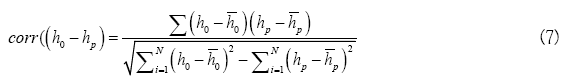
For calibration and evaluation of the model, Root Mean Square Error (RMSE), Mean absolute Error (MAE), and Mean absolute remaining Error (MARE) were used. None of these evaluation criteria can indicate the correctness of modeling independently, and this should be examined using all of them. Even though the correlation coefficient (R) is not an evaluation criterion, it was used, along with other error statistics, to check the coordination between observed and calculated values.

Further, time series graph and simulated and measured values are also suitable for showing calibration and evaluation results in unsteady state.
Results
Steady state results
This step of calibration was used to determine the hydraulic conductivity and total balance of the study area and to create initial conditions for modeling in the unsteady state. Because of the vastness of the study area, the existence of wells and some other characteristics such as the soil texture, the performance of the model required a lot of time in the finite element mode. Hence, the whole hydrological modeling of the basin was done in finite difference mode. Running the model in a steady state took more than 8 days of computational time (3.2 GHz Pentium-4 desktop machine equipped with 4.0 GB RAM).
The observed and calculated water level in observation wells at the end of the steady state is shown in Figure 7. The value of R2=0.96 indicates acceptable accordance between the observed and calculated water table levels and the results can be used as initial condition for running the model in unsteady condition.

Figure 7: Observed and calculated water table in observation wells at the end of the steady state
Unsteady state results
After determining the initial condition, the calibration step of the model was carried out in the period of 1992-2005 for 13 years. The average time needed for each of the model performances at this stage was two days. Due to the existence of multiple variables in the model, complicated relationships and also interactions between surface, subsurface and evaporation, the calibration of the HGS model was difficult. In this step the model was executed more than 200 times using 9 Pentium 4 desktop machine in about 3 months’ period of time and finally the most accurate resulting run was chosen as the result of calibration [30-34].
Tables 2-4 represent the final values of the parameters after calibration. The values of criteria for evaluating the model in unsteady state for observation wells and Koshkabad hydrometric station are presented in Tables 5 and 6, respectively. Also, the time series of the observed and calculated values in calibration and validation steps for observation wells and volume of surface flow are presented in Figures 8 and 9.
| Soil texture | Swr | α | β | Porosity | Specific Yield (%) |
|---|---|---|---|---|---|
| Loam | 0.078 | 0.36 | 1.56 | 0.39 | 4.657 |
| Clay loam | 0.095 | 0.19 | 1.31 | 0.39 | 4.657 |
| Silty loam | 0.067 | 0.2 | 1.41 | 0.39 | 4.657 |
| Sandy loam | 0.065 | 0.75 | 1.89 | 0.39 | 4.657 |
Table 2: Sub-surface flow parameter values (result of calibration)
| Land use | ny (m/s1/3) | nx(m/s1/3) |
|---|---|---|
| Crop and Rangeland | 15 | 15 |
| Garden | 40 | 40 |
| Urban | 3 | 3 |
Table 3: Roughness coefficient values (result of calibration)
| Parameters | Leaf area index | Root depth(m) | Evaporation (m) | C1 | C2< | C3 |
|---|---|---|---|---|---|---|
| Calibrated value | 1.2 | 1.2 | 1.5 | 0.2 | 0 | 12 |
Table 4: Evapotranspiration parameters values (results of calibration)
| No. | Observation well | R | RMSE | MARE | MRE |
|---|---|---|---|---|---|
| 1 | Yengije | 0.94 | 1.99 | 1.60 | -0.04 |
| 2 | Maryanaj | 0.61 | 1.50 | 1.35 | 1.34 |
| 3 | Jade Kermanshah | 0.77 | 1.66 | 1.45 | 0.30 |
| 4 | Salehabad Bahar | 0.89 | 2.51 | 2.03 | -1.66 |
| 5 | Abromand | 0.62 | 0.94 | 0.87 | 0.70 |
| 6 | Salehabad | 0.75 | 1.39 | 1.37 | -1.37 |
| 7 | Bahadorbeyg | 0.66 | 2.82 | 2.23 | 1.52 |
| 8 | Aghche Kharabe | 0.65 | 1.23 | 0.99 | 0.92 |
| 9 | Haroonabad | 0.91 | 5.48 | 4.67 | -1.34 |
| 10 | Hesamabad | 0.94 | 4.23 | 3.20 | 1.63 |
| 11 | Lalejin | 0.98 | 1.45 | 1.22 | 0.53 |
| 12 | Karimabad | 0.90 | 1.92 | 1.58 | -0.40 |
| 13 | Ganjtape | 0.93 | 4.21 | 3.31 | 0.24 |
| 14 | dahangerd | 0.85 | 2.73 | 2.27 | 1.34 |
| 15 | Latgah | 0.93 | 0.72 | 0.60 | -0.05 |
| 16 | Hesaremam | 0.61 | 1.66 | 1.29 | -0.90 |
| 17 | Hasanabad | 0.69 | 1.70 | 1.48 | -1.05 |
| 18 | Dehpiaz | 0.58 | 1.19 | 0.96 | -0.82 |
| 19 | Joraghan | 0.59 | 0.83 | 0.70 | 0.00 |
| 20 | Karkhane Chini | 0.97 | 1.71 | 1.24 | 0.93 |
| 21 | Bahramabad Amzajerd | 0.95 | 4.93 | 4.16 | 1.90 |
| 22 | Dastjerd | 0.96 | 2.77 | 2.47 | -2.22 |
| 23 | Lalejin Jamshidabad | 0.66 | 0.75 | 0.62 | 0.26 |
| 24 | Yeknabad | 0.97 | 2.39 | 2.19 | -1.16 |
| 25 | Hosseinabad | 0.75 | 0.76 | 0.65 | 0.04 |
Table 5: Values of criteria for evaluating the model in unsteady state for observation wells
| Criteria | R | RMSE | MARE | MRE |
|---|---|---|---|---|
| value | 0.96 | 28 | 15.9 | -11.5 |
Table 6: Values of criteria for evaluating the model in unsteady state for Koshkabad hydrometric station

Figure 8a: The observed and calculated values in calibration and validation steps for observation wells

Figure 8b: The observed and calculated values in calibration and validation steps for observation wells

Figure 8c: The observed and calculated values in calibration and validation steps for observation wells

Figure 9: The observed and calculated values in calibration and validation steps for surface flow
Discussion
The evaluation results for observation wells show the acceptable ability of the HGS model in saturated and unsaturated subsurface flow simulation. In some of the observation wells, such as Haroonabad, Hesamabad, and Ganjtapeh, despite the high correlation between observed and calculated values, other evaluation parameters show higher error than other observation wells. This contradiction is due to the high absolute levels of groundwater level changes in these wells. For example, in the Hesamabad observation well, the MARE is 3.20, which in comparison with other wells is somewhat high. But since the total underground water level changes during the simulation period in this well are about 25 meters and the MARE statistic is small in comparison with that, and this cause’s high correlation in this well. As noted above, none of the evaluation criteria can indicate the correctness of modeling independently, and this should be examined using all of them.
According to Figure 9, annual runoff is underestimated in wet years. It is cussed by fixed roughness coefficient which is assumed in the model. In the wet years due to continuous flows, the roughness coefficient decreases in the basin, which ultimately increases the share of runoff in the total balance of the basin.
Conclusion
It is worth noting that despite the acceptable ability of the model to simulate annual runoff of the basin; daily runoff values calculated by the model did not have acceptable agreement with observed values. Error in determining the daily values of evapotranspiration can be the reason for this problem, while these errors at the annual scale will neutralize each other’s effects. However, considering that the purpose of this study is to determine the total balance of water resources in the basin, the model’s ability to predict annual surface flow discharge is sufficient and failure in determining daily runoff can be ignored.
Some of the main sources of error in the calibration step are mentioned bellow:
A- Lack of spatial information about moisture distribution in the unsaturated area in time.
B- Experimental error that is inevitable.
C- The greatest error in the calculation of water table level occurs in marginal observation wells in the aquifer area. According the maps of aquifer these marginal wells were placed out of the aquifer known boundary, then depth of the bed rock was estimated in these areas, and the difference between the estimated and real bed rock levels can be main reason for the error.
REFERENCES
- Hammour ZA, Arqub OA, Momani S, et al. Optimization solution of Troesch's and Bratu's Problems of ordinary type using novel continuous genetic algorithm," discrete dynamics in nature and society. Discrete Dyn Nat Soc. 2014.
- Arqub OA, Hammour ZA, Numerical solution of systems of second-order boundary value problems using continuous genetic algorithm. Inform Sci. 2014;279:396-415.
- Wang HF, Anderson PA. Introduction to ground water modeling. WH Freeman, San Fransisco. 1988.
- Genuchten V, Th M. Closed-form equation for predicting the hydraulic conductivity of unsaturated soils. Soil Science Society of American Journal. 1980;44:892-8.
- Genuchten V, Th M, Nielsen DR. On describing and predicting the hydraulic properties of unsaturated soils. Annals Geophysical. 1985;3(5):615-28.
- Sudicky EA, Jones JP, Park AEY, et al. Simulating complex flow and transport dynamics in an integrated surface subsurface modeling framework. Geosciences Journal. 2008;12:107-22.
- Jones JP, Sudiky EA, McLaren RG. Application of a fully integrated surface-subsurface flow model at the watershed-scale: A case study. Water Res. 2008;44:1-13.
- Cornelissen T, Diekkrüger B, Bogena H. Using hydro geosphere in a forested catchment: How does spatial resolution influence the simulation of spatio-temporal soil moisture variability. Procedia Environ Sci. 2013;19:198–207.
- Cornelissen T, Diekkrüger B, Bogena H. Using high-resolution data to test parameter sensitivity of the distributed hydrological model hydro geo sphere. Water. 2016;8:202.
- Akhavan J, Abedi-Koupai SF, Mousavi M, et al. Application of SWAT model to investigate nitrate leaching in Hamadan–Bahar Watershed, Iran. Agric Ecosyst Environ. 2010;675-88.
- Angel lR, Huff FA. Changes in heavy rainfall in Midwestern United States. ASCE. Journal of Water Resources Planning and Management. 1997;123(4):246-9.
- Therrien R, McLaren ERG, Sudicky A, et al. A three-dimensional numerical model describing fully- integrated subsurface and surface flow and solute transport. HydroGeoSpher. 2010.
- www.hmrw.ir
- Asner GP, Scurlock JMO, Hicke JA. Global synthesis of leaf area index observations: Implications for ecological and remote sensing studies. Global Ecology and Biogeography. 2003;12(3):191-205.
- Brooks RJ, Corey AT. Hydraulic properties of porous media. Hydrology Paper 3, Colorado State University, Fort Collins, CO. 1964.
- Carsel RF, Parrish RS. Developing joint probability distributions of soil water retention characteristics. Water Resour Res. 1988;24:755-69.
- Vázquez RF, Feyen J. Effect of potential evapotrans- piration estimates on effective parameters and performance of the MIKE SHE-code applied to a medium-size catchment. J Hydrol. 2003;270(3-4):309-27.
- Farthing MW, Kees CE, Todd SC, et al. Efficient steady-state solution techniques for variably saturated groundwater flow. Adv Water Resour. 2003;26:833-49.
- Jones JP, Sudiky EA, McLaren RG. Application of a fully integrated surface- subsurface flow model at the watershed-scale: A case study. Water Resour Res. 2008;44:1-13.
- Rasoulzadeh A. Tree-dimensional variably-saturated numerical modeling of groundwater management in a coastal aquifer. Shiraz University. 2006.
- Canadell J, Jackson RB. Ehleringer JR. et al. Maximum rooting depth of vegetation types at the global scale. Ecologies. 1996;108:583-95.
- Li Q, Unger AJA, Sudicky EA, et al. Simulating the multi-seasonal response of a large-scale watershed with a 3D physically-based hydrologic model. J Hydrol. 2008;357(3-4):317-36.
- Chiang WH. 3D groundwater modeling with PMWIN, a simulation system for modeling groundwater flow and transport processes. Springer. 2005.
- Chen Z, Grasby SE, Osadetz KG. Predicting average annual groundwater levels from climatic variables: An empirical model. J Hydrol. 2002;260:102-17.
- Eslamian SS, Khordadi MJ, Abedi-Koupai J. Effects of variations in climatic parameters on evapotranspiration in the arid and semi-arid regions. Glob Planet Change. 2011;78:188-94.
- Feddes RA, Kowalik PJ, Zarandy H. Simulation of field water use and crop yield. John Wiley and Sons, New York. 1978.
- Fowler HJ, Kilsby CG, O’Connell PE. Modelling the impacts of climatic change and variability on the reliability, resilience and vulnerability of a water resource system. Water Resour Res. 2003;39(8):1222-32.
- Hornberger GM, Raffensperger JP, Wilberg PL, et al. Elements of physical hydrology. JUH Press. 1998;312.
- Jones JP. Simulating hydrologic systems using a physically-based surface subsurface model: Issues concerning flow, transport and parameterization. University of Waterloo, Waterloo, Canada. 2005;145.
- Kosugi K. Lognormal distribution model for unsaturated soil hydraulic properties. Water Resour Res. 1996;32(9):2697-703.
- McClave JT, Dietrich FH, Sincich T. Statistics of earth science data: Their distribution in time and space. Statistics. 1997.
- Rasoulzadeh A. Tree-dimensional variably-saturated numerical modeling of groundwater management in a coastal aquifer, Agriculture Faculty, Shiraz University. 2006.
- Rawls WJ, Brakensiek DL, Saxton KE, Estimating soil water properties. ASAE. 1982;25(5):1316-20.
- Sudicky EA, Jones JP, Park Y, et al. Simulating complex flow and transport dynamics in an integrated surface subsurface modeling framework. Geosciences Journal. 2008;12:107-22.