Mathematical formulation of the purchase funnel by using knowledge space theory

Yung-Tzu Lin; Chuan-Yi Chang; Shein-Yung Cheng; Meng-Yun Lin

doi:10.37532/2752-8081.23.7(1).01-19.

Yung-Tzu Lin, Chuan-Yi Chang^*, Shein-Yung Cheng and Meng-Yun Lin

Department of Information and Computer Engineering, Chung Yuan Christian University, Taoyuan City 320314, Taiwan

^*Correspondence: Chuan-Yi Chang, Department of Information and Computer Engineering, Chung Yuan Christian University, Taoyuan City 320314, Taiwan, Email: chang.maverick@gmail.com

Received: 16-Jan-2023, Manuscript No. puljpam-23-6058; Editor assigned: 18-Jan-2023, Pre QC No. puljpam-23-6058(PQ); Accepted Date: Jan 27, 2023; Reviewed: 19-Jan-2023 QC No. puljpam-23-6058(Q); Revised: 20-Jan-2023, Manuscript No. puljpam-23-6058(R); Published: 30-Jan-2023, DOI: 10.37532/2752-8081.23.7(1).01-19.

Citation: Lin YT, Chang CY, Cheng SY et al. Mathematical formulation of the purchase funnel by using knowledge space theory. J Pure Appl Math. 2023; 7(1):01-19.

This open-access article is distributed under the terms of the Creative Commons Attribution Non-Commercial License (CC BY-NC) (http://creativecommons.org/licenses/by-nc/4.0/), which permits reuse, distribution and reproduction of the article, provided that the original work is properly cited and the reuse is restricted to noncommercial purposes. For commercial reuse, contact reprints@pulsus.com

Abstract

The retail industry provides customers with goods or services. Analyzing the purchase behavior of customers is critical for expanding the business. Therefore, managing the repurchase intention of customers is crucial. A sequence of purchase behaviors by each customer constitutes a set of purchase Customer Journeys (purchase CJs), which detail purchase pathways and repurchase behaviors. Purchase CJs are the actual retail transaction data. This study investigated purchase CJs and proposed a purchase funnel called CJ graph (CJG) by measure theory and knowledge space theory with actual retail transaction data. To achieve this objective, a Customer Journey Block (CJB), denoting “touchpoint,” is defined as a series of purchase behaviors during a period and used as the base of this method. Each touchpoint is allotted a measurable function, named Purchase Measure (PM). By integrating all the CJBs of purchase CJs, the Purchase Measure Graph (PMG) can be constructed as the primary structure of the PM knowledge structure. Finally, when all CJs are coordinatized with CJ codes, knowledge space theory is used to develop the Customer Journey Graph (CJG). In this method, knowledge bases are used as the spanning framework of the CJ knowledge space, and the filtering property of the purchase funnel is illustrated. Furthermore, to validate the feasibility of the proposed method, a set of two-year and one million transactions retail data generated from more than thirty-six thousand customers was segmented by Recency, Frequency, and Monetary (RFM) model. Thus, the corresponding PMGs and CJGs of various (12, here) customer segments are detailed, and the resultant knowledge bases of the primary purchases and secondary re-purchases are applied to analyze and predict the customer purchase behaviors accurately.

Keywords

Transaction; Purchase measure; Customer journey; Knowledge space theory

Abbreviations

AIDA Awareness, Interest, Desire, and Action
CJ Customer Journey CJB Customer Journey Block
CJG Customer Journey Graph
EC Equivalence Class
KST Knowledge Space Theory
NB National Brand
PM Purchase Measure
PMG Purchase Measure Graph
PMKS Purchase Measure Knowledge Space
RFM Recency, Frequency, and Monetary
VIP Very Important Person

Introduction

Retail caters to making products available for customers topurchase. However, in a conventional shop floor, when a customer completes the transaction and leaves the store or website, the seller can only hope the customer visits again. Therefore, investigating the customer's repurchase behavior and constructing a model of multiple transactions of customers is critical. In retail, customers buying a certain product is a behavioral tendency of their purchase intention [1]. Repurchase intention or repeat patronage indicates the possibility that customers will repurchase products or avail services of the same brand again [2].

Purchase and repurchase in retailing

Repurchase characteristics

Although repurchase intentions and purchase intentions may appear to be similar consumer behaviors, they have distinct connotations. The purchase intention is a subjective tendency of consumers to consider the purchase behavior, which can be used as a key indicator to predict consumer purchase behavior [3,4]. Repurchase intention is the possibility of customers maintaining the frequency of past consumption and continuing to purchase the same product [5]. In addition to repurchase intension, the customer simultaneously exhibits other behaviors such as word of mouth and public recommendation [6].

Definition of repurchase

When the customer is satisfied with the product or service, then repeated purchase behavior, that is, repurchase intention may occur [7]. Researchers have revealed that customer satisfaction considerably affects purchase intention. High satisfaction positively affects repurchase willingness and can stabilize customers' repeated purchase (repurchase) behavior [8, 9]. The sense of identity is another critical factor. When the customer's sense of identity is higher, they are willing to continue to purchase more products at higher prices. Therefore, a high sense of identity positively influences the willingness to increase prices [10].

Researchers believe that repurchase intentions are “derivative behaviors of loyalty,” which denotes willingness to continue buying and recommending products to others. Therefore, the positive definition of repurchase intention is the derivative behavior of customer loyalty, that is, consumers publicly introduce or recommend to others [11]. For a company, customer loyalty is a critical indicator. The parameter indicates that customers will continue to patronize, repeatedly, or exclusively purchase and use the company's products and services, and introduce the product to their friends [12].

Repurchase model

Increasing customer willingness to buy back is crucial for companies because the finding new customers is approximately five times expensive than retaining existing customers [13,14]. For saving corporate costs, reducing the loss of customers is helpful to the company’s profit than reducing costs [15]. The repurchase intentions of customers can be measured from three aspects, namely:

1.Intents to repurchase: This behavior measures customers’willingness to repurchase the company’s products or services inthe future, which is an indicator of customers’ future behavioralintentions.

2.Primary behaviors: This behavior includes the number ofpurchases, frequency, amount, and quantity of customers.

3.Secondary behaviors: This behavior refers to behaviors thatcustomers help the company introduce, recommend, and buildreputation. Such behaviors are valuable to the company [16].

Among the three behaviors, only primary behaviors can be measured by actual transaction data. For each customer, his/her primary behaviors change over time. Thus, each customer has a distinct CJ.

CJ

CJ characteristics

In general retail purchases, customer experience includes not only the purchase of goods but also the customer’s cognitive, affective, emotional, social, and various physical responses to the purchased brand (service provider) [17]. Furthermore, CJ collects the procedural and empirical aspects from the customer perspectives of these products or services provided by the brand [18]. Formally, this CJ can be described as repeated interactions between customers and the brand (service provider) [19]. Thus, the entire CJ becomes an “engaging story” about the user’s interaction with the brand or can be termed as walking “in the customer's shoes.” [20, 21].

Definition of CJ

The interactions or communications between customers and a brand (service provider) can be defined as “touchpoints” which represents the abstract form of customer experience (the customer's product purchases in this paper) [22-24]. These touchpoints form the building blocks of CJ, which is then described as a series of touchpoints [25-28]. When combined with data analysis, CJ can be visualized as a CJ map [19-20]. The CJ map can be visualized in a stream, in which the touchpoint represents the abstract form of the customer experience (the customer’s product purchases in this paper) [25].

CJ of repurchase

From the perspective of customer purchase analysis, CJ is an open process comparable with the “customer loyalty staircase” [29]. In retail analytics, the evaluation of customer purchase journeys is essential CJ is a clearly defined service process, with marked starting and ending points [30-31]. In the CJ of purchase analysis, the initial touchpoint is the first purchase behavior of a new customer, and the final touchpoint is the purchasing characteristic of loyal customers. Evaluating these topics is essential for researching purchase funnels.

Purchase funnel

Marketing funnel

The relationship between the funnel model and the Awareness, Interest, Desire, and Action (AIDA) was first proposed in the early twentieth century [32]. Marketing funnel theory originates from the hierarchy of effects-based marketing theory, which categorizes the mental state of the consumer into various marketing procedures: from brand awareness, consideration of purchase, to brand preference, and purchase action to achieve brand loyalty [33]. Specifically, consumers performing purchase decisions can be categorized into an AIDA process:

1.Awareness: the customer is aware of the existence of a product or service,

2.Interest: actively express interest in a certain product group,

3.Desire: desire for a specific brand or product,

4.Action: product purchase action [34].

Therefore, using the effect hierarchy of AIDA, the marketing funnel, based on the process of marketing activities and psychological evolution of consumer purchase activities, is used to specifically construct a repeatable, traceable, highly operable customer purchase journey model to improve marketing efficiency.

Conversion funnel

Similar to a marketing funnel, in e-commerce, a “conversion funnel” is used to describe the trajectory of consumers browsing e-commerce websites through Internet advertising or search systems, and finally converting the search into sales [35]. In digital marketing funnel, consumers may find products they desire through advertisements or keyword searches on the web. Subsequently, social media is used to compare prices and consumer reviews to target websites or platforms. However, the purchase may occur in physical stores or online. This shopping experience and after-sales customer service determines if the customer will return. In practice, the marketing funnel, which is a conversion funnel, is a visual interactive tool that represents the key conversion process from sales leads to sale completion. Figure 1 details the conversion ratio of e-commerce stores from online impressions (92,000 people) to actual orders received on the website (42 people). The conversion in each of the two stages provides insights into sales performance. For example, the pay-per-click marketing activities is related to the number of nonrepetitive visitors from online impressions (92,000 people) to the website (more or less than 3,200 people). This process is not limited for only e-commerce. Similar conversion funnels can be used for business-to-business companies or physical retail stores [36].

Figure 1: Conversion funnel of e-commerce

The “purchase funnel,” “sales funnel,” “marketing funnel,” or “customer funnel” is a consumer-focused marketing model that is used illustrate the theoretical CJ of customers purchasing products or services [35]. Studies have investigated multiple stages along the purchase funnel to investigate manufacturers perspective on managing National Brands (NBs) and the influence of instore retailer-specific activities on the purchase decision [37]. Through purchase funnel, data analytics provide insights on customers, such as their behaviors, their incoming channels, and purchased contents [30].

Research objectives

Paper targets

Based on retail transaction data, this study proposed PM theory to construct the theoretical foundation of CJs, developed PM graph and customer journey graph (purchase funnel), and applied actual corporate data applications.

Contributions and objectives

The major contributions of this paper are as follows:

(1) To propose algorithms for the formulation of the Purchase Measure Graph (PMG) and coordinate system to represent customers’ purchase behaviors.

(2) To introduce pseudo-source design to integrate customer journeys into one connected graph and ensure PMG exhibits well-behaved properties.

(3) To define the measurement functions, such as purchase frequency measure μF(.) and/or purchase monetary (the amounts of products) measure μM(.) of customer journey block (CJB), and the equivalence class, which is the purchase measure quotient space for formulating Purchase Measure Knowledge Space (PMKS).

(4) To add quantitative values into the knowledge states of the knowledge space, such as coordinates, volumes, and customer flows of state transitions.

(5) To provide an algorithm for the formal description of Customer Journey Graph (CJG) and to model purchase funnel by using a CJG.

(6) To apply a two-year retail data from over thirty-six thousand customers to prove the feasibility of the purchase funnel and help the marketing strategy of retail business through the study of customer’s purchase journey by formulating the model of “marketing funnel” using the formal method.

Outlines

Section 2 formulates the purchase measures and forms their purchase measure space, Section 3 proposes a Purchase Measure Graph (PMG). By slightly modifying PMGs, Section 3 also introduces the knowledge space theory to develop the purchase measure knowledge space and analyze the corresponding knowledge base. For the knowledge states in the PM knowledge space, Section 4 presents a study of their quantitative values, including the coordinates, volumes, and flows of state transitions. Subsequently, the Customer Journey Graph (CJG or purchase funnel) is developed to visualize its filtering property. To prove the feasibility of the purchase funnel, a two-year retail data from over 36000 customers is used in Section 5 to establish PMGs and CJGs for the exploration of CJs of various customer segments. Section 6 presents the conclusion.

PM SPACE

Customer PM space

Transaction space

Let C = {C_i} be the set of customers, P = {p_j} be the set of products, max M = { m_j : m_j ε [0,M_max ]} be the payment, and the time t ε T , which denotes a time interval. A customer purchase behavior is defined as a quadruple as follows:

equation

which indicates the customer C = {C_i} purchases {P_j } ⊆ P with the expense {m_j} at time t ε T . A transaction space Ξ (C,P,M,T) =C ×2^P×2^M× T encircles all the possible transactions x’s in Equation (1), in which 2^P and 2^M denote the power set of P and M, respectively. The following analysis begins with a transaction set X contained in the transaction space Ξ.

Example 1

When the transaction space is formed from the customer set CA = { c₁, c₂ , c₃, c₄ , c₅} , the product category set PA = { g₁, g₂ , g₃, g₄} , the payment range M_maxA=499999, and the time interval 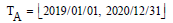equation . Here, g1 - g4 are product categories, and not only products. The illustrated transaction space in Example 1 are presented in Table 1.

TABLE 1 Conversion funnel of e-commerce

Customer	Date	Category	Amount
c₁	1/16/2019	g₁	1990
c₂	7/6/2020	{g₂, g₃}	{3224, 2414}

CJ

CJ is the experience-shaping process by which consumers (c_i) use products and brands (p_j) to fulfill their goals [38]. Geometrically, each customer purchase behavior (c_i, {p_j}, {m_j}, t) in Equation (1) is a scattering of points within the space Ξ (C,P,M) but along the line (c_i, t). In this space, a formal definition of CJ of the retail repurchase process can be formally derived.

Definition 1

Given a customer c_i, his/her customer journey can be extracted from the transaction space as a triplet set:

ξ[c_i {({p_j}, {m_j}, T)} ⊆ 2 ×2×T,∀(c_i , {p_j}, {m_j}, t) with fixed ci, products (services) {p_j } ' s ⊆ P , expense {m_j}’s ⊆ M , and time t ε T

In Example 1, ξ A [c₁]= {g₁,1990, 2019/01/16) , (g₁,2682,2019/06/02) , (g₁,3582, 2019/06/120 , (g₁,261, 2020/04/29) , (g₄ ,3944, 2020/05/08) , ({g₂, g3}, {3224,2414}, 2020/07/06)} . Here, each customer journey ξ[c_i] is defined as a series of customer purchase behaviors within the transaction space

PM

CJB

A CJ is a series of purchase behaviors of a customer. To measure CJ, some measurement duration should be defined first.

Definition 2

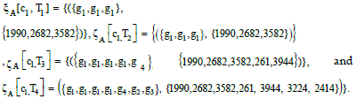
The CJB (CJ block) ξ [c_i ,T_k] is series of measurement durations which transforms the time interval T into a series of time intervals [T_k], in which T_k is the beginning to some timestamp. Next, the set of customer journey blocks is defined as follows:

equation

with products (services) {P_j} 's ⊆ P , payment

Such ξ[c_i ,T_k ] is one kind of touchpoints (CJ building blocks), which collects the customer c_i’s purchase experience within T_k. CJ ξ [c₁]= {ξ [c_i ,T_k ]} is described as a series of touchpoints[ 26,28, 39].

For Example 1, as the time interval TA is segmented into [T₁, T₂, T₃, T₄] = [2019/01/01-2019/06/30, 2019/01/01-2019/12/31, 2019/01/01-2020/06/30, 2019/01/01-2020/12/31], then the aforementioned CJ ξ_A [c₁] can be segmented into

equation

The aforementioned definitions of Tk’s are all counted from the beginning, which ensures the product set is accumulated.

LEMMA 1

∀T_i ⊆ T_j ,ζ[c_i ,T_i ] ⊆ ζ[c_i ,T_i].

Proof

Because T_i ⊆ T_j,T_ji exists such that T_i =T_i T_ji , then,

equation

PM

Irrespective of products (services) or time, a CJ presents an increment phenomenon, which indicates the quantity of its contents (products, services, frequencies or expenses) is increasing. For each CJ segment an ξ[c_i ,T_k0 ], atomic PM λ ({p_j},{m_j}, T_k0)can be defined based on some quantity of the purchase behavior ({p_j},{m_j},t) in Equation (2) during customer ci purchasing within a basic time interval T_k0, such as about:

(1) the amounts / quantities of products (categories), services {p_j},

(2) the frequencies or time about t ∈ T_k0, or (3) the total sums of the expense {m_j}.

Such measure satisfies two properties: (1) λ ({p_j},{m_j}, T_k0)≥ 0 and (2) λ ({p_j},{m_j}, T_k0) = 0 if and only if {({p_j},{m_j}, T_k0)} is an empty set, that is, no purchase within T_k0. Therefore, a measure μ :π → R + ∪{0} can be defined to summarize a description of products (services) or times in a CJ.

Definition 3

The PM of a CJ block ζ[c_i, T_k] is a function mapping from a set of CJBs π in Equation (2) to a non-negative real number, that is, μ :π → R⁺ ∪{0} , and

equation

to aggregate all atomic PMs in this interval Tk.

Applications of purchase measures (PMs)

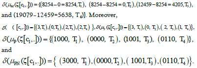
For Example 1, several purchase measures (abbreviated as PMs) μ(.) in Equation (3) can be defined as follows. A PM μ(.) may be a real number, such as the purchase amount of products (services); for example, ( 1,. ) {(1990+ 2682+ 3582= 8254, T₁ , (8254, T₂ , (8254+261+3944=12459, T₃ ) , (12459+3224+2414=18079, T₄ )}. Similarly, μ(.) can be an integer to denote the purchase quantity or frequency. The purchase quantity describes the purchased products (services), for example, and the frequency is a quantitative value of the visit times, for example,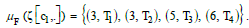 By contrast, μ(.) in Equation (3) can be a logical value that indicates whether the customer purchases the product. For example, 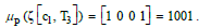A PM can not only be a scalar but also be a vector (collection) of the purchased content, such as the aforementioned 10110, or precisely 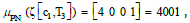in which the numbers indicate the quantities of the purchased products. Not restricted to the aforementioned products, numerous definitions of PMs have been proposed. The use of PM depends on its applications.

PM space

Definition of the PM space

Although PMs can be defined in various methods, they exhibit common properties and can be used to construct the purchase funnel.

LEMMA 2

A PM μ(.) is a (mathematical) measure.

Proof

A PM μ(.) satisfies the three properties of a mathematical measure: (1) non-negativity; (2) null empty set comes from the non-negativity of λ(.), and the vanishing of λ(.) represents no purchase behavior; (3) "countable additivity" of a mathematical measure can be derived from the following equation:

equation

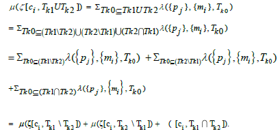
Mathematically, forms a transaction space and its customer journey {ξ[c_i ,T_k ] ={({p_j,{m_j},t)} forms a measurable space (Ξ,ζ). Accordingly, PM μ(.) is a (mathematical) measure on (Ξ,ζ). The triple (Ξ,ζ,μ) forms a measure space, called purchase measure space (PM space).

Properties of PM space

Because PM space (Ξ,ζ,μ) is a standard measure space, a set of basic properties can be derived accordingly.

Proposition1

Defined in the PM space (Ξ,ζ,μ) , the PM μ(.) exhibits the following basic properties of measure space:

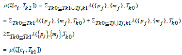
(1) Monotonicity: equation

(2) Subadditivity: 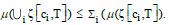equation

Proof

(1) By Lemma 1, the inclusion of Tk1⊆Tk2 reveals that (pj, mj) exists such that 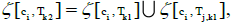equation then we have the following expression:

equation

by Lemma 2.

(2) By countable additivity,

equation

Next, the subadditivity property can be obtained by induction.

For a standard measure space, many other properties, such as continuity from below/above, completeness, additivity, and so on, are not used in our derivation and neglected here.

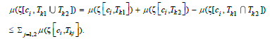
Increment of PMs

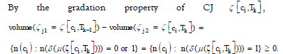
By the monotonicity of the PM μ(.) along a specific customer journey ζ[c_i,T_k], the increment of PMs can be defined as follows:

equation

which denotes the incremental quantity of the PM in touchpoint ζ[c_i,T_k-1] to the next touchpoint ζ[c_i,T_k]. To complete the definition, the initial value is set as δ(μ(ζ[c_i,T₁])=μ(ζ[c_i,T₁]).

From Equation (4), the aforementioned PMs μM(.) can provide

equation

In Section 3, purchase measures, first, are used to construct the PMG. Next, in Section 4, the increment of purchase measures is formally used to investigate the quantitative properties of the PM in CJ.

Pmg and Its Knowledge Analysis

PM quotient space

PM equivalence relation

If values of PM μ(.) are finite, define a PM equivalence relation is defined as equation For the purchase product measure μP(.), a more all-zero-products pseudo-source (0000 in Example 1) is added to treat all customers as new comers. If not, more elaborate designed can be detailed. Thus, μP(.) provides the PM space with n (C) * (n(T)+1) values, where n(C) and n(T) are the sizes of customer set C and time interval set T, respectively.

For μ_P(.) in Example 1, although 5*(4+1)=25 measure values are possible, and the customer c1 has only five elements: 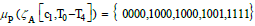equation For the expense measure μ_M(.), quantity measure μ_Q(.), frequency measure μ_F(.), and the product quantity measure μ_PN(.) are used. Infinite measure values are possible and they should be quantified.

PM equivalence class, PM quotient space

With the finite or quantified measure values and their resultant equivalence relation, the equivalence class of PM space and the corresponding quotient space can be defined.

Definition 4

Given the PM space (Ξ,ζ,μ) with finite-valued measure μ(.), a PM equivalence class of (Ξ,ζ,μ) can be defined as follows:

equation

which is the PM quotient space (set) Qμ of Ξ and each [q_k] is a partition of space .

Following the PM μP(.) of ζA[.,.] in Example 1, the corresponding quotient space in Equation (5) can be in which 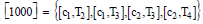with size 4.

Size of the PM quotient space

Similarly, the count of elements in partition Qμ of Equation (5) is denoted as n(Qμ) and is called the size of the PM quotient space, which satisfies the condition: 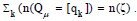For example, 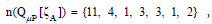whose sum just match the number of elements in ,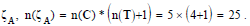

PMG

PM relation

Next, the relation between the elements of PM equivalence classes, which comes from CJ, are evaluated.

Definition 5

Given the PM space and its PM Equivalence Class (EC) equation a PM relation is expressed as follows:

equation

In graph theory, quasi-ordinal is defined as a relation that satisfies reflexivity and transitivity. With this definition, the following theorem can be obtained easily.

Theorem 1

Given the PM space , the PM relation E(Ξ, ζ, μ ) is a quasiordinal relation.

Proof

From Lemmas 1,2 and Proposition 1, T_k⊆T_k+1 makes equation then the PM relations of E(Ξ, ζ, μ )= {(q_i , q_j )} is quasi-ordinal.

PMG

The aforementioned PM EC collects the touchpoints of CJs with similar PM μ(.). Therefore, purchase funnel can be defined as a partial ordering graph.

Definition 6

Given the PM space (Ξ,ζ,μ) and its PM EC Q_μ = [q_k]satisfying Equation (5), a PMG can be defined as , where the vertex set is the PM EC in Equation (5), , and the edge set is in Equation (6).

Combining previous derivation, such PMG can be obtained through the following algorithm.

Algorithm 1. (PMG Algorithm)

Given a PM space , the PMG (Q , E) μ ψ can b e obtained by the following steps:

(1) Find all the customer journeys in Equation (2)

(2) Add pseudo-source to each customer and calculate all the PMs μ (ζ [c_i , T_k ]) in Equation (3).

(3) Divide the measure space Ξ into several ECs Qμ’s in Equation (5), which also forms the vertex set V_set.

(4) Find the edge set Eset in Equation (6) from the consecutive PMs ’s in all the CJs.

(5) Then form the PMG equation .

Because PM measure μ(.) satisfies the property of monotonical increasing, as presented in Proposition 1, the resultant PMG exhibits the partial ordering property.

PMG for example 1

For the construction of PMG in Example 1, the vertex set in Equation (5) is adopted as

equation

and edge set E in Equation (6) can be obtained from the collection of CJs of all customers, such as 0000 →1000 →1001 →1111 from customer c₁. The resultant PMG is displayed in Figure 2.

Figure 2 PMG of Example.

In Figure 2, the CJ block in each vertex (EC) is shortened in a notation sum c_i/T_k, which indicates the aggregation of [c_i,T_k]. For the aforementioned example of [1000]={[c₁,T₂], [c₁,T₃], [c₂,T₃], [c₂,T₄]} is denoted as 1000=1/2+1/3+2/3+2/4 in Figure 2.

Pseudo-source design

With the pseudo-source design in Section 3.1, all the nodes in the PMG ψ(Q_μ , E) originate from the pseudo-source. As displayed in Figure 2, pseudo-source (0000) can integrate all the three components of ψ(Q_μ , E) into one connected graph and causes PMG to exhibit well-behaved properties.

PM knowledge structure

With the partial ordering of PMGs, knowledge space theory (KST) can be used to study the CJ [40].

The aforementioned set of equation is the domain to be processed, such as ζ[c₁ ] = {0000, 1000, 1001, 1111}. Therefore, the basic KST and knowledge structure can be introduced with the PM.

Definition 7

Given a PMG equation a purchase measure knowledge structure, is defined as (ζ, K), where ζ is the domain of CJs and the set of knowledge states K ⊆2^ζ and K ≠ φ (empty set).

In Example 1, ζ_A = {{0000,1000,1111} , {0000, 1011} , {0000,1100,1110} , {0000,1000,1001,1111}}, each of which corresponds to the CJs of {c₂}, {c₃,c₄}, {c₅} and {c₁}. Notably, equation . Moreover, a subset of A ζ such as {0000} → {0000,1000} → {0000,1000,1111} is an element of the PM knowledge structure KA, that is,

Quasi-ordinal knowledge structure

When a knowledge structure K is closed under intersection, such knowledge structure ( ζ⁺, K) becomes a quasi-ordinal relation. To make (ζ, K) quasi-ordinal knowledge structure, those knowledge states equation , where

equation

encircles not only ζ , but their partial paths, that is, the subsets, of 2^Qμ. Such knowledge structure extends the domain set from ζ to .

For example, in addition to equation still contains {0000, 1000}, {0000, 1000, 1111} and the single pseudo-source {0000}. Moreover, such intersection closeness condition of can be described formally.

LEMMA 3

For one quasi-ordinal PM knowledge structure in Equation (7),

equation

Proof

By definition.

PM knowledge space

In mathematics, the construction of a space represents the following: (1) finding the basic elements of this space is possible. Such elements are typically named bases. (2) All the elements in this space can be spanned by the combinations of these “bases.” The spanning logic is always illustrated by a set of “coordinates”.

Definition 8

A PM knowledge structure (ζ⁺ , K) is called a PM knowledge space (ζ⁺ , K^*), where K^* is closed under union, that is,

equation

Such union is a coordinate, which is explained subsequently. The following property occurs naturally.

Proposition 2

Given a PMG ψ_f(Q_μ ,E_f ), the purchase measure knowledge space satisfies equation which reveals that and

Proof

By definition.

With union operations of knowledge states in Example 1, its knowledge space equation can be obtained as follows:

PM knowledge base

According to research, a knowledge space Г(ζ⁺ , K^* ) from Equations (7) and (8) admit at most one knowledge base, called PM knowledge base B_K, which is a minimal family of knowledge states spanning the knowledge space [41]. Such a knowledge base can be found by an “algorithm for constructing knowledge base” and is implemented in a ready-made software [42].

equation

Based on previous research, the PM knowledge base of the PM knowledge space in Example 1 can be equation {{0000}, {0000, 1000}, {0000, 1011}, {0000, 1100, 1110}, {0000, 1000, 1001, 1111}} .

CJs and future prediction

From the perspective of CJ, knowledge base may provide considerable insights. First, the pseudo-source (e.g., 0000) is the staying point of the new customer. Other knowledge bases function as the purchasestarting points of CJ tracks.

In Figure 3 of Example 1, 0000-1000, 0000-1011, and 0000-1100 are the starting points of CJs {c₁, c₂}, {c₃, c₄}, {c₅}, respectively. Notably, the length-2 purchase path 0000-1000-1001-1111 is an extended purchase of 0000-1000 and plays the role of a knowledge base, which is Proof investigated in the following section.

Figure 3 PM knowledge space of example 1

CJG in the Pm Knowledge Space

PM coordinate system and CJG

PM coordinate system

Before spanning the knowledge space by knowledge bases, investigating the knowledge bases is necessary. From the perspective of the coordinate vector space, a basis is a set of independent vectors {β_k}, such as Equation (9), called PM axes, to completely describe (span) the vector space and the PM origin β₀ is the intersection of these bases.

In the PM knowledge base of Example equation are three independent PM vectors (axes), and β_kA0 = 0000 is the origin. Moreover, the PM knowledge base has the PM path of the path length more than one, such as 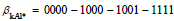, which should be in the direction of β_kA1 = 0000 - 1000.

Therefore, the PM coordinate system can be organized as follows.

Algorithm 2. (Algorithm for PM coordinate system)

The coordinate system A_K={a_k} with respect to (w. r. t.) PM knowledge base B_K={β_k} in Equation (9) can be coded as follows:

1. Coordinate w.r.t. pseudo-source β₀: coded as the origin;

2. Coordinate w.r.t. PM axes β_k: coordinate as a unit dimensional vector a_k,

3. Extended coordinate w.r.t. purchase path extended axes β_k* of path length more than one: coded as the dimensional vector of the path length along axes.

Using this algorithm, the aforementioned PM knowledge base B_KA={{0000}, {0000, 1000}, {0000, 1011}, {0000, 1100, 1110}, {0000, 1000, 1001, 1111}} can be coded as A_KA={[0,0,0], [1,0,0], [0,1,0],[0,0,1],[2,0,0]}.

PM knowledge space spanning

With knowledge base B={β_k} in Equation (9), it is sufficient to reconstruct the full knowledge space as follows:

equation

With PM knowledge base B = {β_k} and its corresponding PM coordinate systems A={a_k}, the PM knowledge space ( ζ⁺ ,K^* ) in Equation (7) and (8) can be easily constructed by ζ⁺ as the using domain of K^* [41].

From the perspective of evolution theory, when customers exchange their purchased information with each other, it causes purchase behavior interaction, which results in mating or mutation in evolution theory. In terms of the knowledge space, a union operation is formed between purchase behaviors, which can be used to predict possible future knowledge states.

CJG

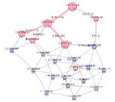
By the partial ordering of the subset property of K^*, the PM knowledge space in Figure 3 is a graph of the Hasse diagram, called CJG.

Definition 9

Given a PMG Ψ_f(Q_μ, E_f) and its PM knowledge space (ζ⁺, K^*) with CJ block in Equation (7) and PM knowledge space K^* in Equation (8), then a CJG of (ζ⁺, K^*) is defined as Г(K^*,Λ), where the vertex set is the PM knowledge space, that is, Vset(Г)=(ζ⁺, K^*), and the edge set is

equation

The resultant CJG equation in Example 1 is displayed in Figure 4, in which each circle keeps a coordinate (000 to 211) and its corresponding customer journey (0000 to 0000, 1000, 1001, 1011, 1100, 1110, 1111).

Figure 4 CJG of Example 1

By knowledge space analysis, these nodes K_A^* in Figure 4 not only represent CJs but also cover the PM knowledge states, which have coordinates in the form of a_k=(x_k,y_k,z_k) where x_k = 0 - 2 and y_k,z_k = 0/1 . Thus, the overall PM knowledge space is a three- dimensional (3D) cube with 3 × 2 × 2 = 12 elements. The x-axis has two unit vectors, 0000 - 1000 and 0000 -1000 -1001 -1111 , coordinated as (1,0,0) and (2,0,0). The unit vectors of y-axis and z-axis are 0000-1011 (with coordinate (0,1,0)) and 0000-1100-1110 (with coordinate (0,0,1)), respectively. These knowledge states in the knowledge base or the knowledge structure are represented as pink or orange circles, respectively.

Furthermore, the rest knowledge states shown in gray circles, for example, 011 (0000,1011,1100,1110) and 201 (0000,1000,1001,1100,1110,1111), are not in any dimensional axis and exhibit the coordinates of more than one digit. Such knowledge states denote mixed CJs and represent the future possible consumption behaviors of these customers.

Volumes and flows in the PM knowledge space

CJ code

Each node of CJG Г(K^* , Λ) of Equation (11) is a knowledge state ζ_i (or μ(ζ_i) precisely) of the knowledge space, which denotes just a customer journey of some customers, such as ζ_A[c₁]= 0000- 1000 - 1001 - 1111. In this example, μ(ζ) are the nodes in the PMG ψ_f(Q_μ ,E_f) , that is, (ψ_fA(Q_μ_A ,E_{f A})) = [000, 1000, 1001, 1011, 1100, 1110, 1111] , representing purchase product patterns (or more precisely product category patterns) at one purchase duration.

By contrast, one customer journey ζ_i in a knowledge state, such as ζ_A [ c₁] , is one purchase pattern, which describes the purchase sequence (0000, 1000, 1001, 1111) along this CJ. Such knowledge state can then be coded as a 0/1-vector corresponding to one purchase product pattern in Vset (ψ (Q_μ , E)).

Definition 10

Given a PMG ψ_f(Q_μ ,E_f) and its corresponding knowledge space (ζ⁺ , K^* ), then for each customer journey (knowledge state) ζ_i ε K^* , its corresponding CJ code (along PMG) is defined as follows:

equation

where equation if elsewhere.

For example, equation and all the nodes in CJG can be coded as 1000000 (0000), 1100000 (0000,1000), …, 1111111 (0000,1000,1001, 1011,1100,1110,1111), which are listed in Table 2, called the codebook of CJ knowledge space. In the first node, the first element in the top node 1000000 indicates 0000, which is pseudo-source and included in all ζ’s nodes.

TABLE 2 Codebook of the CJ knowledge space in Example 1

	0	1000	1001	1011	1100	1110	1111
0	1	0	0	0	0	0	0
0000,1000	1	1	0	0	0	0	0
0000,1011	1	0	0	1	0	0	0
0000,1000,1011	1	1	0	1	0	0	0
0000,1100,1110	1	0	0	0	1	1	0
0000,1000,1001,1111	1	1	1	0	0	0	1
0000,1000,1100,1110	1	1	0	0	1	1	0
0000,1011,1100,1110	1	0	0	1	1	1	0
0000,1001,1000,1011,1111	1	1	1	1	0	0	1
0000,1000,1011,1100,1110	1	1	0	1	1	1	0
0000,1000,1001,1100,1110,1111	1	1	1	0	1	1	1
0000,1000,1001,1011,1100,1110,1111	1	1	1	1	1	1	1

Volume of the knowledge state

To investigate the aforementioned CJG with the node set in Equation (10) and edge set in Equation (11), the volume of a knowledge state is defined as the number of customers in this state ζ_k , symbolized as follows:

equation

For equation in Example 1, volume( [ 1000000, 1100000, 1001000, 1101000, 1000110, 1110001 ])=[5,2,2,0,1,2] and the volumes of the other nodes are all zeros. The top node pseudo-source β₀ possesses the volume n(C), which indicates that all CJs start from the very node.

Flow between knowledge states

When a customer c_i makes a purchase equation in the buying process, the CJ (knowledge state , will switch to another CJ (knowledge state . For customer c1, a more purchase of g₁ in T₁ renders ζ [c₁,. ] from CJ 0000 (knowledge state 1000000) to CJ 0000,1000 (state 1100000). Such knowledge state switching also occurs in ζ [ c₂ ,T₂ ] , which causes an edge flow of 2. Formally, we have the following expression:

equation

for (ζ₁ , ζ₂ ) ε Λ in Equation (11).

Quantitative analysis in CJG

Gradation of CJ

For a CJ ζ [c₁,. ] , gradation is defined as the difference in the touchpoint ζ[ c_i, T_k] from its predecessor ζ[ c_i, T_k_-1] by one item [43]. Equation (4), the gradation represents the vanishing or unit quantity of increment PM as follows:

equation

Which indicates ζ[ c_i, T_k] is the same as the predecessor ζ[ c_i, T_k] (0) or just purchase one-more single product/category (1).

The gradation of CJ indicates that a purchase CJ is a stepwise customer journey, which indicates a single purchase in one touchpoint (CJB), not multiple purchases. The descriptions about PM increments of Example 1 reveal that gradation is not common in customer journey; however, this condition can hold under certain conditions and is highly characterized on the purchase measure.

CJG and its quantities

The volumes and switching flow of the knowledge states were merged into the CJG, whose nodes are encoded as customer journey codes, as displayed in Figure 5. In CJG graph, the paths from the pseudosource to the terminal nodes are the purchase journeys of customers. Each node in the CJG is a knowledge state and denotes a purchase journey of the customer, and the node label is in the form of CJ coding (e.g., 110000) followed by its volume in a parenthesis (e.g., (2)), and the purchased product categories are listed in the following diagram (e.g., 0000,1000).

Figure 5 Quantified CJG of example 1

Quantitative properties of CJG

A CJG includes two knowledge nodes: (1) the nodes in knowledge bases: displayed in red circles in Figure 5, and (2) the nodes in the knowledge space but not in the knowledge base: displayed as gray circles in Figure 5. The edges and paths between two CJ nodes indicate the switching between these two nodes.

Such knowledge state switching exhibits filtering properties in the sense of product purchase and customer volume.

LEMMA 4

Given a customer journey graph Г(K^* , Λ), the nodes (customer journeys) exhibit two filtering properties: (1) the increasing in equation and moreover, for all Eset(Г) = Λ of gradation customer journey graph, (2) the decrease in customer

Proof

(1) By the definition of

equation and make an edge of Eset of Г.

equation

Although Lemma 4 can be proven only for gradation CJs, the decreasing property of customer volumes holds in almost all the conditions.

Conversion rate and CJG algorithm

Based on the node volume in Equation (13) and edge flow in Equation (14), a meaning term, conversion rate, can be defined for each edge (ζ_k1, ζ_k2 ) ε Λ as follows:

equation

With the node volume and edge conversion rate, the aforementioned CJG such as Figure 5 can be developed in a systematic way.

Algorithm 3. (CJG algorithm)

Given the PM space (Ξ, ζ, μ), the customer journey graph (CJG) Г(K^* ,Λ) can be obtained by the following steps:

(1) Construct the PMG (Q_μ , E) ψ using Algorithm 1.

(2) Build up the quasi-ordinal knowledge structure of (ζ⁺ , K) from Equation (7) and Equation (8) with the intersection closure.

(3) Furthermore, find the knowledge space (ζ⁺ , K^*) with union closure.

(4) Find the corresponding knowledge base 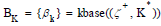in Equation (9).

(5) Let the vertex set K*= {ζ_i } in Equation (10) be the knowledge states of the knowledge space (ζ⁺ , K^* ) , then VL = {volume(ζ_k)} from Equation (13).

(6) For in Equation (11), calculate flow FL = { flow(ζ₁ , ζ₂ )} from Equation (14), and conversion rate CR = {conversion (ζ_k1, ζ_k2)} from Equation (16).

(7) Then the CJG is found as CJG Г(K^* , Λ, VL, FL, CR).

CJG filtering

For Example1, the CJ code of pseudo-source in Figure 5 is 1000000. The path represents customer journey ζ[c₅,.] and the path includes ζ[c₃,.] and ζ[c₄,.]. Then these two paths own flows 1 and 2, respectively, and exhibit conversion rates 1/5=0.2 and 2/5=0.4, respectively. However, the path 10 encircles ζ[c₁,.] and ζ[c₂,.], and the extended path has only one customer c1. Then, the corresponding flows are 2 and 1, respectively, and the conversion rates are 2/5=0.4 and 1/2=0.5, respectively.

This example indicates a direct corollary of Theorem 2. This CJG can also be called a purchase funnel, which occurs from the filtering properties of the CJG.

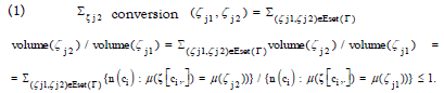
Theorem 2. (CJG Filtering of the purchase funnel)

Given a customer journey graph * Г(K , Λ,V, F , R) constructed using Algorithm 3, the node volumes V in Equation (13) and edge conversion rates R in Equation (16) exhibit the following relationships: (1) Σ_ζj2 conversion (ζ_j1,ζ_j2)≤1 for any node ζ_j1ε K^*.

(2) equation with the first ζ_k1 = ζ_i and the last ζ_k2 = ζ_j.

equation

The definition of the conversion rate renders equation The formula can then be obtained by iterations.

With such filtering properties, the purchase funnel (CJG) can be applied into many applications of retail business, as explained in the following section.

CJG in the Pm Knowledge Space

Real transaction data and its RFM model

Format of real transaction data

This experiment is based on the actual data of retail for big data analysis. The data was obtained from a 40-year retail brand of a company. This brand has cloud e-commerce and approximately 300 physical stores. The company is engaged in the apparel industry, and tops, jackets, shoes, bags, and accessories are top product categories. The brand has more than 40,000 active customers in the past three years.

The data of this experiment was obtained from N=1035056 real transactions in 2019 - 2020 , 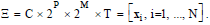equation This data only requires four major categories, namely P={g₁=tops, g₂=skirts, g₃=pants, g₄=dresses }. All the transactions are similar to that in Table 1. An actual transaction owns data attributes more than the four (customer, data, category, amount) attributed in Table 1, in which the necessary data attributes in the present study are adopted.

RFM model

The aforementioned transactions are real buying behaviors generated by Nc=36716 active customers C={ci, i = 1, ..., Nc}. These customers can be partitioned into several groups by customer segmentation, which is a popular tool for identifying various customer groups with similar needs and behaviors [44]. Researchers divide customer segmentation into six categories, namely demographic data, geographic data, psychographic data, attitudinal data, sales data, and behavioral data, in which the visit frequency and monetary volume of sales data constitute the RFM model [45].

In practice, the RFM technique is applied with three terms: (1) recency of customer consumption/purchase (R), (2) purchase frequency over a period of time (F), and (3) purchase amount (monetary) during this period (M) [46]. Such purchase frequency (F) and purchase amount (monetary) (M) is used to classify the 36716 customers, as presented in Table 3.

TABLE 3 RFM mode of experiment data

F\M	0-999	10³-(10⁴ - 1)	10⁴-(10⁵- 1)	10⁵-(10⁶ - 1)	10⁶-(4×10⁶ - 1)	Sum
1	532	9094	1760	0	0	11386
2-9	5	5676	13275	132	0	19088
10-99	0	0	3034	3085	4	6123
100-999	0	0	0	90	29	119
Sum	537	14770	18069	3307	33	36716

In Table 3, purchase frequency (F) is divided into four segments: F=1 for one-time customers, F = 2 ~ 9 indicates 2–9 times for repeated customers, F = 10 ~ 99 denotes 10–99 times for frequent customers, and F = 100–9999 denotes 100–999 times for very frequent customers. By contrast, purchase amount (M) is divided into five segments: equation , and corresponding to customers who consume several hundred NT$ (new Taiwan dollars), thousands of NT$, tens of thousands of NT$, hundreds of thousands of NT$, and customers of more than one million NT$, respectively, in two years (2019-2020) . Thus, 4 × 5 = 20 customer segments were possible, in which eight segments were empty.

Customer values and customer value segment

In Table 3, purchase frequency (F) and amount (M) are used to segment 36716 customers into 12 (=20-8) nonempty customer segments. Because customers in various segments exhibit distinct contribution to business, Table 3 is called the customer value table.

Formally, the customer value is the perception attitude of customers toward giving and getting and is related to the customer's attributes of the product and the goal or purpose that the customer wants to achieve [47, 48]. For the actual operation of customer relationship management, the customer value segments in Table 3 provides several observation points:

(1) A total of 119 customers visit more than 100 times within two years, and the total consumption amount exceeds 100,000 NT$, which can be the threshold of being Very Important Person (VIP).

(2) A total of 11386 one-time customers constituted nearly 31% of total customers.

(3) A total of 19088 repeat customers visited 2–9 times, of which 13275 customers spent 10,000 to 100,000 NT$. These customers were the main consumers.

(4) The spending of frequent customers who visited 9 times-99 times was evenly distributed between tens of thousands NT$ and hundreds of thousands NT$; however, four customers had a spending power of millions NT$.

In the following, these customer value segments are used to analyze the knowledge space of CJ.

These customer value segments are used in the following subsections to analyze the knowledge space of CJ.

PMG/CJG of frequency customers

Transaction Data to the PMG

When PMG and CJG were investigated by the frequency customers of F=9-99 and M ≥ 1Ã¢??10⁵, a comprehensive details of CJGs was obtained. First, the 5056 transactions of 132 customers who visited 9-99 times and spent more than 10,000 NT$ were obtained to conduct knowledge space analysis of CJ. As discussed, the two-year (2019-2020) transactions are categorized into four time intervals [T1,T2,T3,T4]=[2019/01/01-2019/06/30,2019/01/01-2019/12/31, 2019/01/01-2020-06-30,2019/01/01-2020/12/31] and then each PM is in the form of [g1,g2,g3,g4]. Thus, this indicates whether the customer purchased these four product categories in the time interval Tk, k=1,..,4.

Algorithm PMG can be used to generate the corresponding PMG, as displayed in Figure 6, and Figure 6 adopts 9 PM ECs {0000, 1000, 1100,.., 1111} as its vertex set. The edges denote the directions of purchase journeys. Note that the value under purchase measure, for example, the number 4 under 1101, represents the number of elements in the PM EC.

Figure 6 Purchase measure graph of 132 returning valuable customers

When self-loops are neglected, Figure 6 can form a partial ordering set, with the pseudo-source 0000 as the top node and 1001, 1010, 1101, and 1111 as the bottom nodes. To ensure such CJs obvious, the knowledge space analysis is helpful.

Knowledge space analysis and the CJG

Given Figure 6 as the PMG, Algorithm CJG can be used to generate a sophisticated CJG, as displayed in Figure 7. In a CJG, the knowledge bases are displayed in pink circles. Each knowledge state node is labeled with the CJ code, volume, and the corresponding PM. For each edge between two states, the conversion rate and customer flow are also labeled.

Figure 7 Customer journey graph (CJG) of 132 returning valuable customers

Data insights of Figure 7

The subgraph in Figure 7 corresponding to those pink nodes depicts the structure of knowledge bases. Two main branches of the primary knowledge bases exist: nearly 60% customers (59.1%) purchase g1 (1000) in the following choice, and only a small part of customers (1.5%) purchase g1, g3, and g4 next. The first branch (110000000) then continues to purchase g2, g3, or g4 with different probabilities (80.8%, 21.8% and 3.8%). Moreover, customers buying g1 and g2 are probably (with probability 1.6%) make more complete (g3 and g4) purchase. The knowledge base structure provides a probabilistic description of the knowledge space of the entire customer purchase journey.

Knowledge analysis of customers with different customer value segments

PMGs of different customer value segments

For the customer value table in Table 3, all the 12 customer segments in the customer value model were considered, the resultant PMGs from Algorithm PMG and their nodes are arranged in Table 4. Because the customer numbers in the last monetary segment 10⁶ ~ 4 .10⁶ are small, they are combined with the previous number (10⁵-(10⁶ -1)).

TABLE 4 Various customer segments and their PMGs

No.	F (frequency)	M (monetary )	No. of customers	purchase measures (nodes)
(A)	1	0-999	532	0000, 0010, 0100, 1000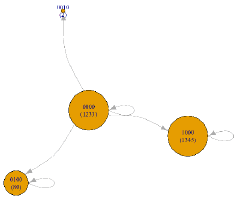
(B)	1	10³-(10⁴-1)	9094	0000, 0001, 0010, 0011, 0100, 0101, 0110, 1000, 1001, 1010, 1011, 1100, 1110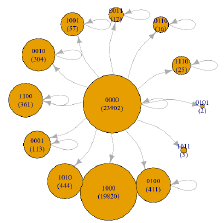
(C)	1	10⁴-(10⁵-1)	1760	0000, 0001, 0010, 0011, 0100, 0101, 0110, 0111, 1000, 1001, 1010, 1011, 1100, 1101, 1110, 1111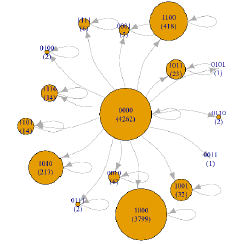
(D)	2-9	0-999	5	0000, 1000
(E)	2-9	10³-(10⁴-1)	5676	0000, 0001, 0010, 0011, 0100, 0101, 0110, 1000, 1001, 1010, 1011, 1100, 1101, 1110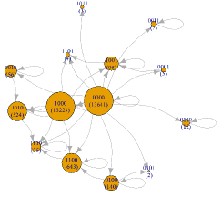
(F)	2-9	10⁴-(10⁵-1)	13275	0000, 0001, 0010, 0011, 0100, 0101, 0110, 0111, 1000, 1001, 1010, 1011, 1100, 1101, 1110, 1111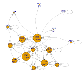
(G)	2-9	10⁵-(10⁶-1)	132	0000, 1000, 1001, 1010, 1011, 1100, 1101, 1110, 1111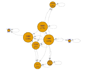
(H)	10-99	10⁴-(10⁵-1)	3034	0000, 0001, 0010, 0100, 1000, 1001, 1010, 1011, 1100, 1101, 1110, 1111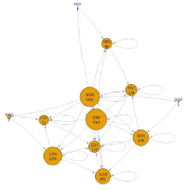
(I)	10-99	10⁵-(4×10⁶-1)	3085+4	0000, 0010, 0100, 1000, 1001, 1010, 1011, 1100, 1101, 1110, 1111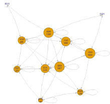
(J)	100-999	10⁵-(4×10⁶-1)	90+29	0000, 1000, 1010, 1100, 1101, 1110, 1111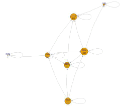

Table 4 reveals that for one-time customer and repeat customer visiting 2–9 times, the corresponding PMGs are simple ring structures, especially for those customer segments with ten thousand NT$ (10⁴ -1). These simple CJs originate from the lowvisit frequency and sparse purchased product categories. The largest one-category purchase is g1 (1000) and the largest two-category purchases are (g1, g2) and (g1, g3), with 1100 and 1010, respectively.

CJGs of different customer value segments

Customers with consumption amount more than ten thousand NT$ have more complex purchase journey, which should be explored by Customer Journey Graph (CJG, purchase funnel). For customer segments with monetary amounts greater than 10000 (10⁴), Table 5 lists all the Frequency (F), Monetary (M), customer number, customer journey codes, knowledge states, and the resultant CJGs. Each bit in a knowledge state of Table 5 corresponds to one PM in the customer journey code, for example, the second bit in knowledge states of the first data row (row (A)) denotes the 0001 PM.

TABLE 5 Various Customer Segments and their CJGs

No.	F (frequency)	M (monetary )	No. of customers	customer journey code w.r.t. purchase	(Customer journey) knowledge state	Purchase Funnel(Customer Journey Graph, CJG)
No.	F (frequency)	M (monetary )	No. of customers	customer journey code w.r.t. purchase	(Customer journey) knowledge state	Purchase Funnel(Customer Journey Graph, CJG)
(A)	2-9	10⁴-(10⁵-1)	13275	0000, 0001, 0010, 0011, 0100, 0101, 0110, 0111, 1000, 1001, 1010, 1011, 1100, 1101, 1110, 1111	1000000000000000, 1100000000000000, 1000010000000000, 1000000010000000, 1011000000000000; 1010000010000000; 1000100010000000; 1010000011100000; 1000100011001000; 1000101010101000; 1000000111111111ÃÃÂ??Â ÃÃÂ??Â ÃÃÂ??Â ÃÃÂ??Â ÃÃÂ??Â ÃÃÂ??Â ÃÃÂ??Â ÃÃÂ??Â ÃÃÂ??Â ÃÃÂ??Â ÃÃÂ??Â ÃÃÂ??Â ÃÃÂ??Â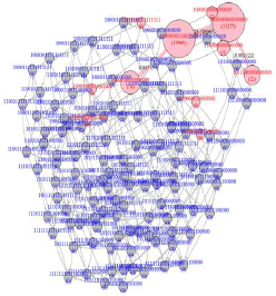
(B)	10-99	10⁵-(10⁶-1)	132	0000, 1000, 1001, 1010, 1011, 1100, 1101, 1110, 1111	100000000, 110000000, 111000000, 110100000, 110001000, 100001100, 110011011
(C)	10-99	10⁴-(10⁵-1)	3034	0000, 0001, 0010, 0100, 1000, 1001, 1010, 1011, 1100, 1101, 1110, 1111	100000000000, 110010000000, 101010000000, 100110000000, 100110001000, 100011100000, 100010101000, 100010111111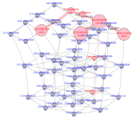
(D)	10-99	10⁵-(4×10⁶-1)	3085+4	0000, 10000, 0010, 0100, 1000, 1001, 1010, 1011, 1100, 1101, 1110, 1111	10000000000, 10010000000, 11010000000, 10110000000, 10011100000, 10011001000, 10010101000, 10011111111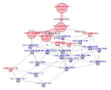
(E)	100-999	10⁵-(4×10⁶-1)	90 +29	0000,1000, 1010, 1100, 1101, 1110, 1111	1000000, 1100000, 1001000, 1110000, 1101111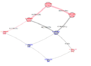

Data insights of Table 5

Several observations can be made from these purchase funnels:

(1) As designed initially, all CJs originated from the pseudo-source (knowledge state with customer journey 0000).

(2) For the CJGs in Table 1-5 and 2 primary knowledge bases with different customer journeys were present, in which these purchase journeys with g1 (1000) were mostly the largest volumes 10968, 78, 667+2462+6+2, 1589 and 24+94, respectively. Here, g1 in the third and fifth CJGs mix with other product categories.

(3) CJGs not only exhibited the primary purchasing product category but the secondary or even the third product categories, shown as those knowledge states with path lengths≥2.

(4) Comparing CJGs of More Valuable Customers (MVCs, with F=2-9 and M = 10⁵ ~ (10⁶ -1) ) in row (B) and more frequent customers (MFCs, with F=10-99 and M = 10⁴ ~ (10⁵ -1) ) in row (C). According to CJGs, MFCs have diversified in their primary purchasing products (110010000000, 101010000000, 100110000000 and 100011100000); whereas, MVCs ensure a more concentrated primary purchase (59.1% for g1 with 11000000 coding), and subsequent differentiate with other three secondary purchasing categories.

(5) The last CJG (in row (E)) of the customers with the most frequent visits and most valuable amount illustrate the final mature purchase patterns, in which approximately 20% customers will purchase g1 and 80% customers purchase g1 and g2 simultaneously.

Because these CJs originate from two-year transactions, longer data may provide complete results. Commercially, three-year data are always used.

Knowledge analysis of VIPs

Customer frequency and monetary measures

In the experiments, the actual retail transaction data is used to develop PMGs and CJGs with purchase product measure μ_P(.). In the following, the research point turns to the construction of the PMG/CJG with other purchase measures, such as purchase frequency measure μ_F(.) and/or purchase monetary (the amounts of products) measure μ_M(.).

Here, both of these two measures are considered with (1) 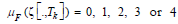equation for the values of visiting frequency , respectively; and (2) 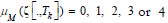for the values of purchased amount monetary (ζ ([.,T_k ])) falls in 0, 0-999, 1000-9999, 10000-99999, 100000- 999999, and 1000000-3999999, respectively. Next, 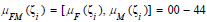is a combined measure of μ_F(.) and μ_M(.), such as μ_F_M(.)=23 means frequency (ζ [.,T_k ] ) = 2 - 9 and monetary equation

From the customer value table in Table 3, the customer value segments of 90 VIPs customers with F=100-999 and M=100000-999999 are selected in the following customer journey study.

PMG of VIPs with purchase frequencies/monetary measures

Because these 90 customers are VIPs, they generate 21545 transactions in two years and generate abundant information about purchase journey. According to the approach of this study, seven ECs (vertices), namely 00, 11, 13,23, 33, 34, and 44, exist with each owning 93, 1, 1, 4, 8, 182, and 161 elements numbers, respectively. From the partial ordering property of CJs, the switching from one PM to another PM is used to generate the PMG, as displayed in Figure 8. By the essential nature of VIPs, the source and destination nodes of Figure 8 are 00 (the node of no consumption) and 44 (the node of F=100-999 frequency and M=100000-999999 consumption), respectively.

Figure 8 Purchase frequency/monetary measure graph of VIPs

CJG of VIPs with purchase frequencies/monetary measures

To systematically study CJ, Algorithm CJG was used to generate a knowledge space of CJG, as displayed in Figure 9. The knowledge bases in Figure 9 illustrate two development paths of VIPs: (1) 10 customers from pseudo-source (00) directly jump into 23, 33 (consuming 10000-9999 in 10-99 times), then 6 out of 10 customers develop into VIPs (31). (2) A small part (2) customers exhibit slow consumption 11 to 13 (once with 1000-9999 consumption) in the beginning.

Figure 9 CJG of VIPs with purchase frequency/monetary measures

Although only 10+2 customers are present in these two basic consumptions (knowledge bases), all other customers consume in mixed styles. These customers with suitable components (coordinates) can be located, as derived in Section 4.

Conclusion

Summary

This study provides a strong theoretical foundation of CJs. Furthermore, PM graph and CJG (purchase funnel) were established to investigate the repurchase behavior in retail transactions. For repurchase, CJ and purchase funnel of retailing, Section 1 details their definitions, characteristics, and conceptual model to provide a research background. Section 2 derives the mathematical formulation of PMs and forms the PM space. Furthermore, Section 3 presented a set of purchase measure ECs and detailed construction of PMG. Section 3 removes the self-loops of a PMG, finds its terminal nodes to form partial ordering, which is used to perform the knowledge space analysis for the knowledge base of CJ. Section 4 provides quantitative values of the knowledge states of the knowledge space, such as the coordinates, the volumes, and the customer flows of state transitions. Thus, a CJG was obtained on filtering the information. This is called the purchase funnel. Furthermore, the theoretical derivation and illustrated example of purchase funnel is presented, and a complete two-year transaction data of actual retail business is presented in Section 5. Several PMGs and CJGs were established to investigate CJs effectively.'

Future works

In this study, the corresponding PMGs and CJGs of various (12, here) customer segments were detailed, and the resultant knowledge bases of the primary purchases and secondary re-purchases were applied to analyze and effectively predict customer purchase behaviors. This study provides a theoretical basis for the knowledge space analysis of CJ. Future studies can focus on numerous avenues. Section 4 details the coordinates, volumes, and customer flows for obtaining CJG. Numerous knowledge states properties can be investigated in the future. The derivation of the knowledge states was obtained from Algorithms 1.28 and 1.31, whose calculation require considerable computation time and should be improved. Such applications require effective algorithms. Finally, the feasibility of these two graphs, PMGs and CJGs, should be detailed in the retail business.

Funding

No Funding

Author Contribution

These authors contributed equally to this work.

Conflict of Interest

The authors declare that they have no known competing financial interests or personal relationships that could have appeared to influence the work reported in this paper.

References

- Dodds WB, Monroe KB, Grewal D. Effects of price, brand, and store information on buyers’ product evaluations. J Mark Res. 1991;28(3): 307–19.
- Tsiros M, Mittal V. Regret: A model of its antecedents and consequences in consumer decision making. J Consum Res. 2000;26:401–17.
- Keller KL. Building customer-based brand equity. Mark Manag. 2001;10:14–21.
- Monroe KB. Pricing: Making profitable decisions McGraw Hill. 1990; 2nd ed.
- Davidow M. Organizational responses to customer complaints. What works and what doesn't. J Serv Res. 2003;5(3):225–50.
- Jones TO, Sasser WE. Why satisfied customers defect. Harv Bus Rev. 1995;73(6):88–99.
- Francken DA. Postpurchase consumer evaluation, complaint actions and repurchase behavior. J Econ Psychol. 1983;4(3):273–90.
- Cronin JJ, Taylor S. Measuring service quality: A re-examination and extension. J Mark. 1992;56(3):55–68.
- LaBarbera PA, Mazursky D. A longitudinal assessment of consumer satisfaction/dissatisfaction: The dynamic aspect of the cognitive process. J Mark Res.1983;20(4):393–404
- Fullerton G. The impact of brand commitment on loyalty to retail service brands. Can J Adm Sci. 2005;22(2):97–110.
- Hunt KA, Keaveney SM, Lee M. Involvement, attributions, and consumer responses to rebates. J Bus Psychol. 1995;9(3):273–97.
- Lovelock CH, Wright LK. Principles of service marketing and management. Prentic-Hall. 2002.
- Kotler P. Marketing management. Prentice-Hall.2003; 11th ed.
- Reichheld FF, Sasser WE. Zero defections: Quality comes to services. Harv Bus Rev.1990;68(5):105–11.
- Kotler P. Marketing management: Analysis, planning, implementation and control (9th ed.). Prentice Hall Coll Inc. 1994.
- Gronholdt L, Martensen A, Kristensen K. The relationship between customer satisfaction and loyalty: Cross-industry differences. Total Qual Manag. 2000;11(4–6):509–14.
- Verhoef PC, Lemon KN, Parasuraman A, et al. Customer experience creation: Determinants, dynamics and management strategies. J. Retail. 2009;85(1):31–41.
- Folstad A, Kvale K. Customer journeys: A systematic literature review. J Serv Theory Pract. 2018;28(2):196–227.
- Meroni A, Sangiorgi D. Design for services. Gower. 2011.
- Stickdorn M, Schneider J. This is service design thinking: Basics, tools,cases. BIS Publishers. 2010.
- Holmlid S, Evenson S. Bringing service design to service sciences, management and engineering. Serv Sci Manag Eng Educ 21st Century. 2008;3:341-45.
- Patrício L, Fisk RP, Cunha JF, et al. (2011). Multilevel service design: from customer value constellation to service experience blueprinting. J Serv Res. 2011;14(2):180–200.
- Zomerdijk LG, Voss CA. Service design for experience-centric services. J Serv Res. 2010;13(1):67–82.
- Zomerdijk LG, Voss CA. NSD processes and practices in experiential services. J Prod Innov Manag. 2011;28(1):63-80.
- Diana C, Pacenti E, Tassi R. Visualtiles: Communication tools for (service) design. In Proc ServDes. 2009;65–76.
- Clatworthy S. Service innovation through touch-points: development of an innovation toolkit for the first stages of new service development. Int J Des. 2011;5(2):15–28.
- Gloppen J. Service design leadership. In Proc ServDes. 2009;77–92.
- Kankainen A, Vaajakallio K, Kantola V, et al. Storytelling group–a co-design method for service design. Behav Inf Technol. 2012;31(3):221–30.
- Nichita ME, Vulpoi M, Toader G.Knowledge management and customer relationship management for accounting services companies. In Proc Eur Conf Knowl Manag. 2012;12(6):435-42).
- Kaila S. How can businesses leverage data analytics to influence consumer purchase journey at various digital touchpoints?. J Psychosoc Res. 2020;15(2):699–714.
- Whittle SR, Foster M. Customer profiling: getting into your customer's shoes. Manag. Decis. 1991;27(6).
- Townsend W W. Bond salesmanship. H. Holt. 1924.
- Lavidge RJ, Steiner GA. A model for predictive measures of advertising effectiveness. J Mark. 1961;25:59–62.
- Lewis EE. Financial advertising. (The history of advertising). Levey Brothers. 1908.
- Jansen BJ, Schuster S. Bidding on the buying funnel for sponsored search campaigns. J Electron Commer Res. 2011;12(1):1–18.
- Runthecompany. Sale Funnel tools and insights. Retrieved from. Accessed June 24, 2020.
- Lamey L, Deleersnyder B, Steenkamp JE, et al. New product success in the consumer packaged goods industry: A shopper marketing approach. Int J Res Mark. 2018;35(3):432–52.
- Hamilton R, Price LL. Consumer journeys: developing consumer-based strategy. J Acad Mark Sci. 2019;47(2):187–91.
- Gloppen J. Perspectives on design leadership and design thinking and how they relate to European service industries. Des Manag J. 2009;4(1):33–47.
- Doignon JP, Falmagne JCl. Spaces for the assessment of knowledge. Int J Man-Mach Stud. 1985;23(2):175–96.
- Doignon JP, Falmagne JC. Knowledge spaces. 1999.
- Stahl C, Meyer D, Hockemeyer D. Package ‘kst’. 2022.
- Doignon JP, Falmagne JC. Knowledge spaces and learning spaces. Tech rep. 2015.
- Abbasimehr H, Bahrini A. An analytical framework based on the recency, frequency, and monetary model and time series clustering techniques for dynamic segmentation. Expert Syst Appl. 2021;192:116373.
- Griva A, Bardaki C, Pramatari K, et al. Retail business analytics: Customer visit segmentation using market basket data. Expert Syst Appl. 2018;100:1–16.
- Hughes AM. Strategic database marketing: The masterplan for starting and managing a profitable, customer-based marketing program. Probus Pub. Co. 1994.
- Zeithaml VA. Consumer perceptions of price, quality and value: A means-end model and synthesis of evidence. J Mark.1988;52(3):2–22.
- Woodruff RB. Customer value: The next source of competitive advantage. J Acad Mark Sci. 1997;25:139–53.