Simulating Ion Trap Quantum Computers

Received: 20-Feb-2023, Manuscript No. puljmap-23-6151; Editor assigned: 22-Feb-2023, Pre QC No. puljmap-23-6151; Accepted Date: Mar 16, 2023; Reviewed: 27-Feb-2023 QC No. puljmap-23-6151; Revised: 07-Mar-2023, Manuscript No. puljmap-23-6151; Published: 23-Mar-2023, DOI: 10.37532.2022.6.1.1-20

Citation: Shaw A. Simulating ion trap quantum computers. J Mod Appl Phys. 2022; 6(2):1-20.

This open-access article is distributed under the terms of the Creative Commons Attribution Non-Commercial License (CC BY-NC) (http://creativecommons.org/licenses/by-nc/4.0/), which permits reuse, distribution and reproduction of the article, provided that the original work is properly cited and the reuse is restricted to noncommercial purposes. For commercial reuse, contact reprints@pulsus.com

Abstract

An ion trap quantum computer is simulated with an exponential speed-up using the Stroboscopic Exponentiation Algorithm (SEA). It leverages Hamiltonian periodicity for time-efficient quantum simulation.

Key Words

Quantum Simulation, Ion Trapping, Quantum, Error Correction

Introduction

Richard Feynman postulated the principle of quantum supremacy: quantum computers possess an innate computing advantage over classical computers [1].

Ion Trap Quantum Computing

Ion trap quantum computers (Figure 1) were proposed by Ignacio Cirac and Peter Zoller in May 1995 [2]. Ion trap quantum computers were experimentally demonstrated by Christopher Monroe et al. in December 1995 [3]. Ion trap quantum computers are the primary market competitors for transmon quantum computers [4–6].

Figure 1: An ion trap quantum computer is composed of ions (black) confined using electromagnetic fields (rainbow). The electronic states are manipulated using lasers (purple)

Ion Trapping

An ion trap confines charged atoms to a spatial region using timedependent electromagnetic fields [7–18].

Quantum operations

Atomic qubits are pairs of electronic states associated with each ion (Figure 2) [19]. Lasers can induce transitions between the electronic states [20–29].

Figure 2: An atomic qubit is composed of a spin-down (left) and spin-up (right) electronic state

Ion trap quantum computers

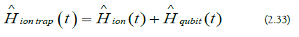
The Hamiltonian for an ion trap quantum computer is derived from quantum theory [30,31].

Ion Trap Hamiltonian

Ionic Hamiltonia

The ion trap parameters are the following:

Atomic Number: Z                      (2.1)

Ion Charge: Qe                         (2.2)

Ion Mass: M                              (2.3)

Number of Ions: N                     (2.4)

a) Kinetic Interactions: The ionic kinetic energy operator is the following [32]:

b) Ionic Interactions: The ionic electrostatic operator is the following [33]:

c) Trapping potential: The trap electric field is the following [8]:

The trap scalar potential is the following [34]:

The trapping operator is the following:

Over a timescale the trapping operator can be approximated by a confining operator [35–37]:

d) Ion-laser interaction: The laser electric field is the following:

The laser magnetic vector potential is given by the following [38]:

The laser magnetic field is the following:

The laser scalar potential is the following:

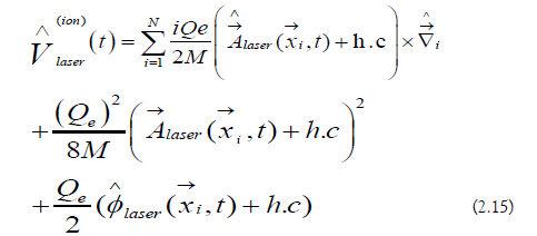
The ionic laser operator is the following:

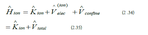
e) Ionic Hamiltonian: The ionic Hamiltonian is the following:

Electronic Hamiltonian

a) Electron number: The number of electrons in the trap is the following:

b) Kinetic Term: The electronic kinetic energy operator is the following:

c) Atomic well: The atomic well operator is the following:

d) Electronic interactions: The electronic electrostatic operator is the following:

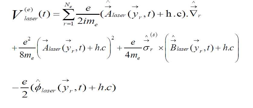
e) Electron-laser interactions: The electronic laser operator is the following [39]:

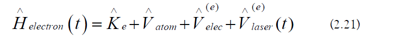
f) Electronic Hamiltonian: The electronic Hamiltonian is the following:

Qubit Hamiltonian

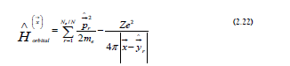
a) Qubit States: The atomic orbital Hamiltonian for a single ion at is the following [40]:

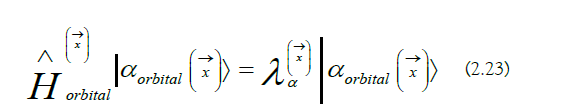
The atomic orbital Hamiltonian’s eigenstates form a complete basis centered at x^→ :

The qubit states are the following (Figure 2):

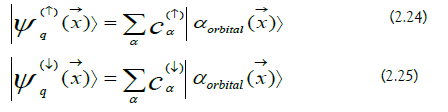
b) Passenger-Qubit Hilbert Space: The passenger-qubit Hilbert space at x^→ is spanned by two states:

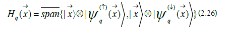
In the passenger-qubit construction, the qubit states co-move with the ion (Figure 3).

Figure 3: The spin-down (left panel) and spin-up (right panel) qubit states vary with the ion position

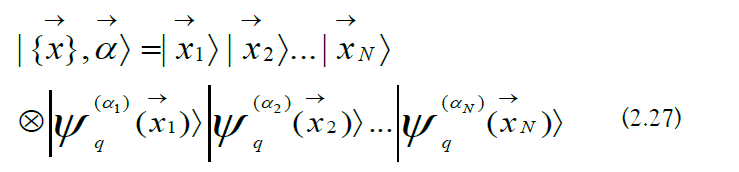
c) Passenger-Qubit Basis States: In the multi-ion case, the passengerqubit basis states are the following:

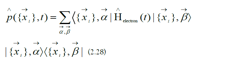
d) Qubit Operators: Qubit operators are projections of the electronic Hamiltonian into the passenger-qubit Hilbert space) To avoid an adiabatic effective Hamiltonian description, a passenger-qudit Hilbert space is required for hyperfine qubits [41-43].

e) Pauli Decomposition: The generalized Pauli operators are the following [44]:

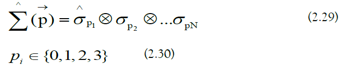
The qubit operators are decomposed in the generalized Pauli basis [45]:

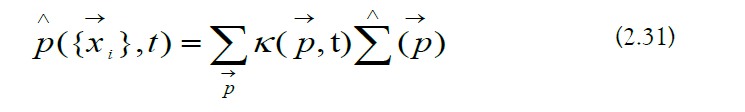
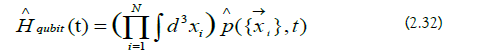
f) Qubit Hamiltonian: The qubit Hamiltonian is the following:

Ion Trap Hamiltonian

Vibrational Expansion

The vibrational expansion approximates the near equilibrium ion trap dynamics by collective oscillatory motion [46].

Vibrational Expansion

a) Total Ionic Potential Energy: In the absence of the laser, the ionic Hamiltonian is expressed using the total ionic potential energy operator:

b) Ionic Component Vector: The ionic position components are thefollowing:

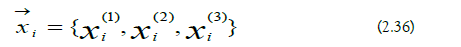
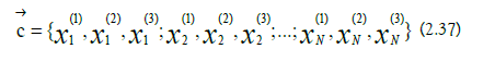
They are used to form the ionic component vector:

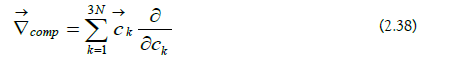
c) Component Gradient: The component gradient is the gradient with respect to the ionic component vector:

d) Critical Point: A critical point of the total ionic potential energy occurs at c₀^→:

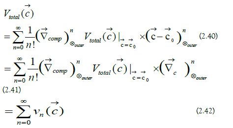
The vibrational expansion is made by expanding the total ionic potential energy around c₀^→:

e) Potential Hessian Matrix: The second-order contribution to the vibrational expansion is expressed as a matrix equation:

The potential Hessian matrix is the following [9]:

f) Trap Frequencies: The potential Hessian matrix is diagonalized as follows:

The eigenvalues of the potential Hessian matrix provide access to the trap frequencies:

Ladder Hamiltonian

a) Vibrational Mode Vector: The vibrational mode vector is the following (Figure 4):

The ions oscillate collectively (red ←→ green) in the ion trap (blue). The center-of-mass mode (left) and the zig-zag mode (right) are shown [42].

b) Harmonic Interactions: The second-order contribution to the vibrational expansion is written in harmonic form:

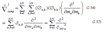
c) Component Laplacian: The component Laplacian is the following:

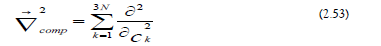
The first partial derivative is expressed in terms of the vibrational mode vector components (Equation 2.49):

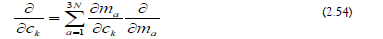
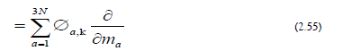
The component Laplacian is the following:

d) Kinetic Interactions: The ionic kinetic energy operator is the following:

e) Ionic Hamiltonian: The ionic Hamiltonian is the following:

f) Mode Ladder Operators: The mode ladder operators are the following [47]:

g) Ladder Hamiltonian: The ionic Hamiltonian becomes the following, up to an overall constant:

The ionic Hamiltonian can be expressed in terms of the physical trap frequencies [48]:

Effective Ion Trap Hamiltonian

Effective approximations are used to tailor the ion trap Hamiltonian for quantum computing applications [49].

Strong−Confinement Approximation

The Strong-Confinement Approximation (SCA) is the following (Figure 5):

Figure 5: If the ion (gray) is strongly confined, the total potential energy (blue) can be approximated (red)

The effective ionic Hamiltonian is as follows:

Weak−Laser Approximation

The Weak-Laser Approximation (WLA) is as follows (Figure 6)

The effective ion trap Hamiltonian is the following:

Figure 6: If the laser (blue) is sufficiently weak, its effect on the ionic wavefunction (left) can be neglected (right)

Interaction Picture Hamiltonian

Interaction Picture

The interaction picture leverages the effective ionic Hamiltonian’s analytic evolution operator for faster computation [50].

a) Interaction Picture Hamiltonian: The effective interaction picture Hamiltonian is the following:

Spin−Phonon Interactions

a) Phonon Passenger-Qubit Basis: The phonon passenger-qubit basis states are as follows:

b) Spin-Phonon Operators: The spin-phonon operators are projections of the electronic Hamiltonian into the phonon passengerqubit Hilbert space:

The effective interaction picture Hamiltonian is written explicitly:

Classical quantum-simulation algorithms

An algorithm is proposed to efficiently simulate ion trap quantum computers.

Product-Formula Algorithms

Product-Formula Algorithms (PFAs) are a family of quantumsimulation algorithms [51, 52]. The PFA is an extremely versatile algorithmic framework, with mathematical, low-energy, and highenergy physics applications [53-82].

PFAs can be represented schematically in three stages:

PFAs can be represented schematically in three stages:

1. Discretization: Subdivide the simulation time into subregions.

2. Piece-wise Simulation: Approximate the subregion evolution operators.

3. Matrix Multiplication: Take the ordered product of the sub-region evolution operators.

Evolution Operator

a) Hamiltonian Operator: The Hamiltonian is the following:

b) Time-Ordered Exponential

Discretization

a) Sub-Regions: The simulation time τ is subdivided into L_sim sub regions:

b) Sub-Region Evolution Operators: The sub-region evolution operators are the following:

The evolution operator can be written as an orderedproduct of the sub-region evolution operators:

c) Piece−Wise Simulation: An intermediate simulation algorithm is used to generate the approximate sub-region evolution operators:

d) Matrix Multiplication: An ordered-product is used to generate the approximate evolution operator:

Time-Integrated Product-Formula Algorithm

The Time-Integrated Product-Formula Algorithm (TI-PFA) coarsegrains the Hamiltonian to minimize the number of required subregions [83–85].

Time−Integrated Product−Formula Algorithm

TI-PFA can be represented schematically in three stages:

1. Time-Averaging: Time-average the Hamiltonian over the sub-regions.

2. Matrix Exponentiation: Generate the approximate subregion evolution operators.

3. Matrix Multiplication: Take the ordered product of the approximate sub-region evolution operators.

a) Time-Averaging: The sub-region Hamiltonians are as follows (Figure 7):

Figure 7: The simulation time is discretized (top) and for each sub-region (blue) the Hamiltonian is time-averaged)

b) Matrix Exponentiation: The approximate sub-region evolution operators are the following:

c) Sub-Region Evolution Operator Error: The eigenvalue spread is as follows (Equation 3.1). The notation max τ indicates a maximum taken over time τ.

The sub-region error coefficient is the following:

The error in the sub-region evolution operators is given by the Baker Campbell-Hausdorff formula [86]:

Quantum-Simulation Computational Cost

The computational cost of TI-PFA is determined by counting the number of elementary operations [87].

Matrix Exponentiation

The approximate sub-region evolution operators are computed using a Λ-truncated Taylor series [88]

The number of matrix multiplications required for the computation is the following:

Matrix Multiplication

Classical computers perform matrix multiplication by manipulating matrix elements:

The number of elementary operations required in the textbook matrix multiplication algorithm is as follows [87]:

The time-complexity is the length of time required for a computing algorithm to run to completion [87]:

Computational Cost

a) Matrix Exponentiation Cost: The computational cost of approximating all of the sub-region evolution operators is the following:

b) Matrix Multiplication Cost: The computational cost of generating the ordered product is the following:

c) Algorithm Cost: The computational cost of TI-PFA is the following:

Quantum−Simulation Error

a) Algorithm Error: The error in TI-PFA is the following (Equation 3.13):

If the discretization condition holds, TI-PFA will achieve the target simulation error reliably:

b) Minimum Algorithm Cost: The perturbative noise condition must hold for TI-PFA to converge (Equation 3.13):

The perturbative noise condition sets the minimum step-number:

The minimum step-number is used to lower-bound the computational cost of TI-PFA (Equation 3.21):

Stroboscopic exponentiation algorithm

The Stroboscopic Exponentiation Algorithm (SEA) leverages Hamiltonian periodicity for time-efficient quantum-simulation.

Stroboscopic Simulation

1. Periodic Hamiltonians

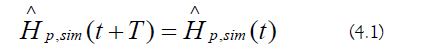
A periodic Hamiltonian has discrete time-translational symmetry with period T:

2. Stroboscopic Evolution Operator

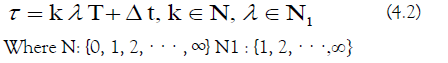
The simulation time can be expressed as follows:

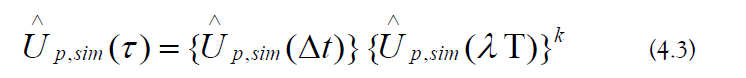
The periodic evolution operator obeys the following [89]:

3. Stroboscopic Simulation Algorithm

The stroboscopic simulation algorithm (SSA) can be represented schematically in two stages (Figure 8) [90]:

Figure 8: The periodic evolution operator is generated for one period (yellow). The base time-symmetry evolution operator (pink) and the time-symmetry evolution operator (green) are generated using matrix multiplication

1. Aliasing: Obtain the base time-symmetry evolution operator and the remainder evolution operator.

2. Matrix Multiplication: Generate the periodic evolution operator using ordered products.

a) Aliasing: The base time-symmetry evolution operator is the following:

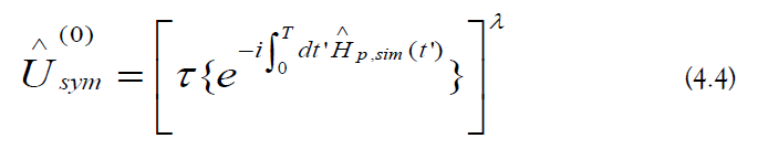
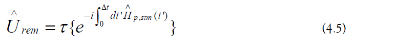
The remainder evolution operator is the following:

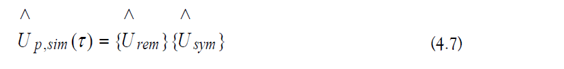
b) Matrix Multiplication: The time-symmetry evolution operator is the following:

The periodic evolution operator is the following:

4. Computational Cost

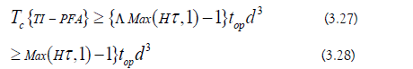
a) Aliasing Cost: The base time-symmetry evolution operator and the remainder evolution operator are both approximated with TI-PFA (Equation 3.28):

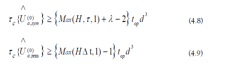
b) Matrix Multiplication Cost: The computational cost of generating the ordered product is the following:

c) Minimum Algorithm Cost: The computational cost of SSA is lower-bounded by the following:

d) Parametrized Minimum Algorithm Cost: The computational cost of SSA can be parametrized as follows (Equation 4.2):

e) Quantum−Simulation Error: The error in SSA is the following (Equation III.23):

Stroboscopic Exponentiation Algorithm

1. Stroboscopic Evolution Operator

The simulation time can be expressed as follows:

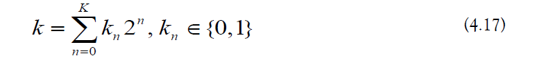
The integer k is expressed using binary notation [91]

The periodic evolution operator obeys the following:

2. Stroboscopic Exponentiation Algorithm

SEA can be represented schematically in three stages (Figure 9):

Figure 9: The exponentiated time-symmetry evolution operators are generated recursively (left). The binary decomposition (right) is used to generate the timesymmetry evolution operator (bottom).

1. Aliasing: Obtain the base time-symmetry evolution operator and the remainder evolution operator.

2. Exponentiation: Perform recursive multiplication on the base time-symmetry evolution operator.

3. Matrix Multiplication: Generate the periodic evolution operator using ordered products.

a) Aliasing: The base time-symmetry evolution operator and remainder evolution operator are defined in Section 4 A 3 a.

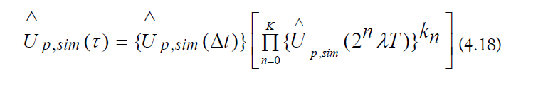
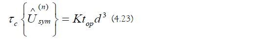
b) Exponentiation: The exponentiated time-symmetry evolution operators are the following:

The exponentiated time-symmetry evolution operators are generated recursively:

c) Matrix Multiplication: The time-symmetry evolution operator is as follows:

The periodic evolution operator is the following:

3. Computational Cost

a) Aliasing Cost: The base time-symmetry evolution operator and the remainder evolution operator are generated as in Section 4 A 4 a)

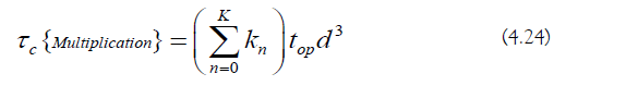
b) Exponentiation Cost: The computational cost of generating the exponentiated time-symmetry operators is the following:

c) Matrix Multiplication Cost: The computational cost of generating the ordered product is the following:

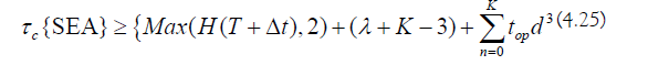
d) Minimum Algorithm Cost: The computational cost of SEA is lower-bounded by the following:

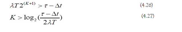
e) Binary Constraint: The binary decomposition constrains the number of exponentiated time-symmetry operators:

f) Parametrized Minimum Algorithm Cost: The computational cost of SEA can be parametrized as follows:

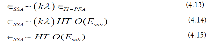
Quantum−Simulation Error

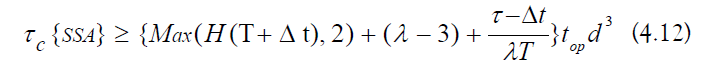
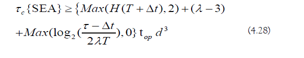
The error in SEA is the following (Equation 4.15)

Algorithm Comparison

Asymptotic Cost Analysis

The asymptotic computational costs of the quantum simulation algorithms are the following:

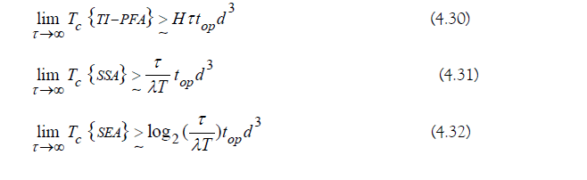
Relative Algorithm Performance: SEA achieves an exponential speed-up over TI-PFA and SSA in simulating periodic Hamiltonians (Figure 10).

Figure 10: The computational cost required to apply TI-PFA (blue), SSA (green), and SEA (red) to a 10-qubit periodic Hamiltonian is empirically determined

Trap sim ii

Trap Sim II

Trap Sim II is a proprietary MATLAB code that performs timeefficient quantum-simulation of ion trap quantum computers.

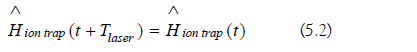
A) Hamiltonian Periodicity

1. Schrodinger Picture Hamiltonian

The laser period is the following:

The Schrodinger picture Hamiltonian is periodic:

2. Interaction Picture Hamiltonian

The interaction picture Hamiltonian is not periodic in general (Equation 2.73).

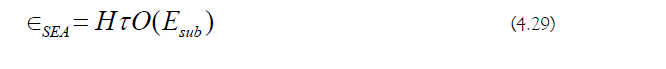
B) Regularization Effects

1. Hamiltonian Regularization

A bosonic truncation is placed on the ladder operators [92–94]:

The regularized effective ion trap Hamiltonian is the following (Equation 2.68):

2. Computer Memory

The dimension of the Hilbert space is the following:

The memory required to perform quantum-simulation on a 64-bit processor is the following (Figure 11):

Figure 11: The threshold simulation memory (black) is compared with the random access memory of several classical computing platforms (colored) [96-98]

3. Bosonic Saturation

The vibrational occupation operators are as follows [95]:

The vibrational occupation uncertainties are as follows:

If the bosonic truncation is saturated, an accumulation of regularization effects ensure that the simulation can no longer be compared to nature:

C) Anisotropic Randomized Truncation

Anisotropic Randomized Truncation (ART) is used to estimate the size of regularization effects. It can be represented schematically in three stages:

1. Truncation: Regularize the Hamiltonian randomly.

2. Quantum-Simulation: Generate an evolution operator for the regularized Hamiltonians.

3. Error-Estimation: Estimate the regularization effects using quantum channel technology.

1. Truncation

The vibrational modes are regularized anisotropically (Figure 12):

Figure 12: The maximum number of vibrational excitations (colored) is set independently for each mode

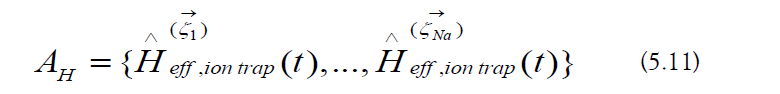
Regularized Hamiltonians are selected pseudorandomly to generate the ART Hamiltonian set:

2. Quantum−Simulation

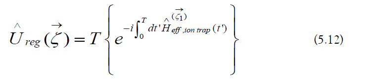
a) Regularized Evolution Operators: The regularized evolution operators are the following:b

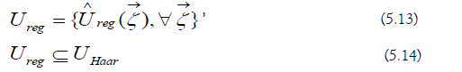
b) Haar Measure: The regularized Haar measure is a subset of the Haar measure composed of the regularized evolution operators (Figure 13) [96-100]:

Figure 13: ART generates unitary operators (red) from the regularized Haar measure (gray), which contains the ideal evolution operator (blue).

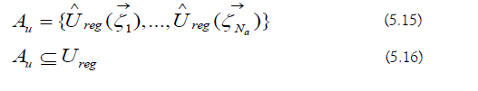
The ART unitary set is the following:

3. Error−Estimation

Simulated Expectation-Value Approximate Reconstruction (SEAR) is used to approximate the regularization effects [101].

a) Quantum Channel Technology: A superoperator on a Hilbert space H has the following form [102]:

A quantum channel is a type of super operator. Its Kraus operators satisfy the following condition [103,104]:

The action of a quantum channel on a state |ψ⟩ generates a density matrix [105, 106]:

b) Quantum Channel Averaging: Applying a similarity transformation to a quantum channel yields the following [107]:

Averaging a quantum channel over the Haar measure yields a depolarizing channel (Figure 14) [107, 108]:

Figure 14: The SEAR error channel (left) is defined using its kraus operators (blue). Averaging the SEAR error channel generates a depolarizing channel (right).

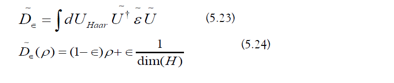
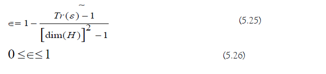
The depolarizing channel has characteristic noise strength [109–116]:

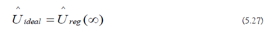
c) Approximate Quantum Simulation: The ideal evolution operator has an arbitrarily large bosonic truncation (Figure 13):

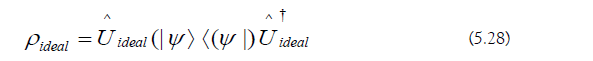
The ideal output state is the following:

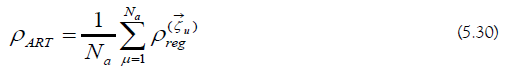
The regularized output states are the following:

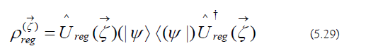
Averaging the regularized output states generated by the ART unitary set yields the ART output state:

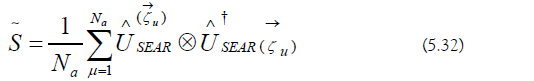
d) SEAR Error Channel: The SEAR error channel maps the ideal output state to the ART output state:

The SEAR error channel is written explicitly:

The SEAR noise strength is the following:

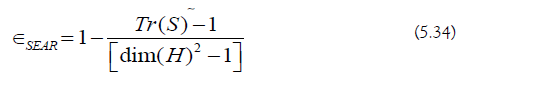
e) Regularization Effects: The SEAR error channel forces observables to stray from their ideal values, causing truncation fluctuations:

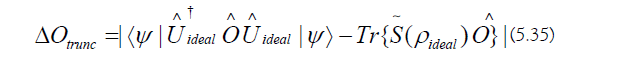
The average truncation fluctuation can be bounded using the SEAR noise strength [101]:

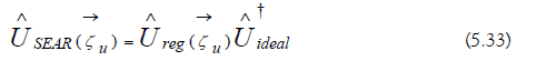
f) Noise Spectroscopy: The complementary SEAR error channels are generated by substituting the ideal evolution operator with the regularized evolution operators (Equation 5.33). The SEAR error channel cannot be studied directly due to the inaccessibility of the ideal evolution operator:

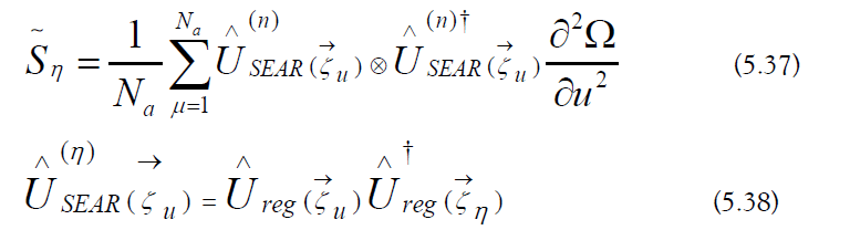
The complementary SEAR noise strength can be estimated using measurement protocols [101, 108].

D) Numerical Results

Trap Sim II is used to simulate an ion trap quantum computer.

a) Simulation Goals: The simulation is performed to examine the following

1. Bosonic Saturation

2. Regularization Effects

3. Entanglement Growth

4. Weak-Laser Approximation (WLA)

b) Simulation Parameters: The simulation parameters are the following [42, 43]:

Number of Ions: N = 1                                      (5.39)

Ion Charge: Q = +e                                           (5.40)

Ion Mass: M ∼ 200 GeV                                    (5.41)

Physical Trap Frequency:                                (5.42)

Laser Wavelength: λ ∼ 400 nm                         (5.43)

Laser Power: P_laser ∼ 1 W                             (5.44)

Bosonic Truncation: ζ ∼ 6                                 (5.45)

Trap Potential: XY-Symmetric & Harmonic           (5.46)

c) Numerical Results

Bosonic Saturation: The vibrational occupation is computed throughout the simulation (Figure 15-16).

Figure 15: On the laser timescale, the vibrational occupation of the X-mode (magenta), the Y-mode (yellow), and the Z-mode (cyan), fluctuates nontrivially around zero.( The uncertainty is amplified by a factor of 104. The observable is sampled 7.5 times faster than displayed))

Figure 16: The vibrational occupation of the modes grows until the bosonic truncation (red) is approached) The onset of bosonic saturation (yellow backdrop) results in unphysical oscillations of the vibrational occupation. (The uncertainty is suppressed by a factor of 3. The observable is sampled 7.5 times faster than displayed).

Computational Details:

The ion trap is initialized in the motional groundstate [117–134]

Regularization Effects: The SEAR noise strength is approximated using ART (Figure 17-18).

Figure 17: On the laser timescale, the SEAR noise strength (green) is perturbative small, indicating the initial accuracy of the quantum-simulation protocol. (The uncertainty is amplified by a factor of 8 × 10⁴ . The observable is sampled 3 times faster than displayed).

Figure 18: The SEAR noise strength (green) approaches unity after the onset of bosonic saturation (yellow backdrop), indicating the ultimate failure of the quantum-simulation protocol. (The uncertainty is amplified by a factor of 5 × 10² . The observable is sampled 3 times faster than displayed).

Computational Details:

• Eight anisotropic bosonic truncations are chosen.

• The SEAR noise strength is estimated repeatedly.

• A bootstrap algorithm is used to generate uncertainty in the average SEAR noise strength estimate [135, 136].

c) Entanglement Growth: The von Neumann entanglement entropy of the qubit is computed throughout the simulation (Figure 19-20). Entanglement entropy is a wildly important quantity, with applications to many areas of physics [137–193].

Figure 19: On the laser timescale, the entanglement entropy (blue) fluctuates non-trivially as the qubit interacts with the vibrational modes. (The uncertainty is amplified by a factor of 2. The observable is sampled 6 times faster than displayed)

Figure 20: The entanglement entropy (blue) ceases to grow after the onset of bosonic saturation (yellow backdrop), and the decoherence of the qubit is halted) (The observable is sampled 6 times faster than displayed).

Computational Details:

• The qubit is initialized in 102 pseudo-randomly generated pure states [104].

• A bootstrap algorithm is used to generate an uncertainty in the average entanglement entropy.

d) Effective Hamiltonian Validity: The WLA error is computed (Figure 21-22).

Figure 21: Over the laser timescale, the WLA error (golden) increases by several orders of magnitude) (The observable is sampled 6 times faster than displayed).

Figure 22:The WLA error (golden) fluctuates non-trivially after the onset of bosonic saturation (yellow backdrop). (The observable is sampled 6 times faster than displayed)

Computational Details:

• The qubit is initialized in 102 pseudo-randomly generated pure states.

• The Pauli operator is measured)

• A bootstrap algorithm is used to generate an uncertainty in the average WLA error.

4. Empirical Observations

a) Bosonic Saturation: After the onset of bosonic saturation, the vibrational occupation exhibits unphysical behavior (Figure 16). Commentary:

• Bosonic saturation places a temporal limit on the amount of ion trap dynamics that can be probed numerically.

• This suggests that ion trap quantum-simulation be used as a performance heuristic for quantumsimulation protocols [194].

• The (N, , ) ζ ∈ ion-trap performance heuristic is the following:

A quantum-simulation protocol passes the (N, , ) ζ ∈ ion-trap performance heuristic by performing quantum-simulation of the Nion, ζ-cutoff ion trap Hamiltonian until bosonic saturation is observed, with total error bounded by∈.

b) Regularization Effects: The noise strength increases with simulation time, and experiences a sharp growth during the onset of bosonic saturation (Figure 18).

Commentary

• Each ART Hamiltonian generates a different set of regularization effects due to the anisotropic bosonic truncation

• The SEAR noise strength provides a measure of the disparity between the ART unitary operators

(Equation 5.33).

• The ART unitary operators diverge during bosonic saturation, and the average error grows to ≥60%.

c) Entanglement Growth: The entanglement entropy of the qubit increases with simulation time until the onset of bosonic saturation. The entanglement entropy then fluctuates non-trivially (Figure 20).

Commentary:

• The entanglement entropy is expected to increase as the purity of the qubit is lost to the environment [195–201].

• Bosonic saturation restricts the decoherence times that can be probed numerically [202-236]:

Decoherence cannot be observed numerically unless the qubits are sufficiently noisy.

d) Effective Hamiltonian Validity: WLA accumulates1% error after the onset of bosonic saturation (Figure 22).

Commentary:

• The stability of approximations such as the rotating-wave approximation, the Lamb-Dicke limit, and the Magnus Expansion may be uncertain in the parameter regimes required for the most ambitious ion trap quantum computing proposals [237–246]. Much of the pressing uncertainty is rooted in the intractability of the Magnus Expansion [247].

• To conserve the limited and transient resources available to the scientific community at large, it is necessary to verify that perturbative protocols will succeed when implemented on real ion trap quantum computers, which are inherently nonperturbative) For a successful instance of this paradigm, see [248, 249].

•Trap Sim II is a rigorous algorithm test-bed for up to six ions (Figure 11). The sole approximation made by Trap Sim II is that of finite bosonic truncation

Appendix

TI-PFA vs. Sampling PFA

The sampling product-formula algorithm (S-PFA) [50, 90] can be expressed schematically in two stages:

1. Sampling: Sample the Hamiltonian at set times and approximates the sub-region evolution operators.

2. Matrix Multiplication: Take the ordered product of the approximate sub-region evolution operators.

a) Sampling

The sub-region Hamiltonians are as follows (Equation 3.9):

The approximate sub-region evolution operators are the following:

b) Sub-Region Evolution Operator Error

The maximum eigenvalue derivative of the Hamiltonian is the following:

c) Relative Algorithm Performance

S-PFA struggles to resolve the true dynamics of the Hamiltonian due to sampling errors , which are not present in TI-PFA [83-85].

Regularization Effects

If the length-scale of the laser is sufficiently long, the severity of the regularization effects can be determined rigorously via an efficient classical computation [250].

Acknowledgement

Unjustly condemned, he was led away.

No one cared that he died without descendants, that his life was cut short in midstream. But he was struck down for the rebellion of my people.

References

1. Feynman RP. Simulating physics with computers. In Feynman comput.  2018: 467(1982); 133-153.

   [Googlescholar]

2. Cirac JI and Zoller P. Quantum computations with cold trapped ions. Phys. rev. lett. 1995; 74(20):4091.

   [Googlescholar] [Crossref]

3. Monroe C, Meekhof DM, King BE, et al. Demonstration of a fundamental quantum logic gate) Physical review letters. 1995; 75(25): 4714.

   [Googlescholar] [Crossref]

4. Gyenis A, Di Paolo A, Koch J, et al. Moving beyond the transmon: Noise-protected superconducting quantum circuits. PRX Quantum. 2021; 2(3): 030101.

   [Googlescholar] [Crossref]

5. Houck AA, Schreier JA, Johnson BR, et al. Controlling the spontaneous emission of a superconducting transmon qubit. Physical review letters. 2008; 101(8): 080502.

   [Googlescholar] [Crossref]

6. Richer S, Maleeva N, Skacel ST, et al. Inductively shunted transmon qubit with tunable transverse and longitudinal coupling. Physical Review B) 2017; 96(17): 174520.

   [Googlescholar] [Crossref]

7. Dehmelt HG. Radiofrequency spectroscopy of stored ions I: Storage) InAdvances at. mol. phys. 1968; 3: 53-72.

   [Googlescholar] [Crossref]

8. Paul W. Electromagnetic traps for charged and neutral particles. Rev. mod) Phys. 1990; 62(3): 531.

   [Googlescholar] [Crossref]

9. Meyrath TP and James DF. Theoretical and numerical studies of the positions of cold trapped ions. Phys. Lett. A) 1998; 240(1-2): 37-42.

   [Googlescholar] [Crossref]

10. Cirac JI and Zoller P. A scalable quantum computer with ions in an array of microtraps. Nature) 2000; 404(6778):579-81.

    [Googlescholar] [Crossref]

11. Kielpinski D, Monroe C and Wineland DJ. Architecture for a large-scale ion-trap quantum computer. Nature) 2002; 417(6890):709-11.

    [Googlescholar] [Crossref]

12. Li MS, Rao XX, Wang Z, et al. Homogeneous linear ion crystal in a hybrid potential. Quantum Inf. Process. 2022; 21(2):65.

    [Googlescholar] [Crossref]

13. Siegele-Brown M, Hong S, Lebrun-Gallagher FR, et al. Fabrication of surface ion traps with integrated current carrying wires enabling high magnetic field gradients. Quantum Sci. Technol. 2022; 7(3):034003.

    [Googlescholar] [Crossref]

14. Lindvall T, Hanhijarvi KJ, Fordell T, et al. High-accuracy determination of Paul-trap stability parameters for electric-quadrupole-shift prediction. J. Appl. Phys. 2022; 132(12):124401.

    [Googlescholar] [Crossref]

15. Burton WC, Estey B, Hoffman IM, et al. Transport of multispecies ion crystals through a junction in an RF Paul trap. ArXiv. 2022.

    [Googlescholar] [Crossref]

16. Miao SN, Zhang JW, Zheng Y, et al. Second-order Doppler frequency shifts of trapped ions in a linear Paul trap. Physical Review A) 2022; 106(3):033121.

    [Googlescholar] [Crossref]

17. Zhang J, Chow BT, Ejtemaee S, et al. Spectroscopic Characterization of the Quantum Linear-Zigzag Transition in Trapped Ions. ArXiv. 2022.

    [Googlescholar] [Crossref]

18. Mihalcea BM. Quasienergy operators and generalized squeezed states for systems of trapped ions. Ann. Phys. 2022; 442:168926.

    [Googlescholar] [Crossref]

19. James DF. Quantum dynamics of cold trapped ions with application to quantum computation. 1997.

    [Googlescholar]

20. Sørensen A and Mølmer K. Entanglement and quantum computation with ions in thermal motion. Physical Review A) 2000; 62(2):022311.

    [Googlescholar] [Crossref]

21. Steane A, Roos CF, Stevens D, et al. Speed of ion-trap quantum-information processors. Physical Review A) 2000; 62(4):042305.

    [Googlescholar] [Crossref]

22. Leibfried D, DeMarco B, Meyer V, et al. Experimental demonstration of a robust, high-fidelity geometric two ion-qubit phase gate) Nature) 2003; 422(6930):412-5.

    [Googlescholar] [Crossref]

23. García-Ripoll JJ, Zoller P and Cirac JI. Speed optimized two-qubit gates with laser coherent control techniques for ion trap quantum computing. Physical Review Letters. 2003; 91(15):157901.

    [Googlescholar] [Crossref]

24. Day ML, Low PJ, White B, et al. Limits on atomic qubit control from laser noise) npj Quantum Inf. 2022; 8(1):72.

    [Googlescholar] [Crossref]

25. Sutherland RT, Yu Q, Beck KM, et al. One-and two-qubit gate infidelities due to motional errors in trapped ions and electrons. Physical Review A) 2022; 105(2):022437.

    [Googlescholar] [Crossref]

26. Martínez-García F, Gerster L, Vodola D, et al. Analytical and experimental study of center-line miscalibrations in Mølmer-Sørensen gates. Physical Review A) 2022; 105(3):032437.

    [Googlescholar] [Crossref]

27. Duan LM. Robust gate design for large ion crystals through excitation of local phonon modes. ArXiv. 2022.

    [Googlescholar] [Crossref]

28. Sutherland RT, Srinivas R and Allcock DT. Individual addressing of trapped ion qubits with geometric phase gates. Physical Review A) 2023; 107(3):032604. 

    [Googlescholar] [Crossref]

29. Yum D and Choi T. Progress of quantum entanglement in a trapped-ion based quantum computer. Curr. Appl. Phys. 2022.

    [Googlescholar] [Crossref]

30. Hamilton WR . On a general method in dynamics; by which the study of the motions of all free systems of attracting or repelling points is reduced to the search and differentiation of one central relation, or characteristic function. Philos. trans. R. Soc  Lond 1834 ;( 124):247-308.

    [Googlescholar] [Crossref]

31. Hamilton WR. Second essay on a general method in dynamics. Philos. Trans. R. Soc Lond 1835; 125:95-144.

    [Googlescholar]

32. Schrödinger E) An undulatory theory of the mechanics of atoms and molecules. Physical review. 1926; 28(6):1049.

    [Googlescholar] [Crossref]

33. Coulomb CA) Memoirs on electricity and magnetism. Chez Bachelier, bookseller; 1789.

    [Googlescholar] [Crossref]

34. Lagrange and Joseph Louis. Artworks by Lagrange) Ministry of Public Education 1867:4
35. Kovacic I, Rand R and Mohamed Sah S. Mathieu's equation and its generalizations: overview of stability charts and their features. Appl. Mech. Rev. 2018; 70(2).

    [Googlescholar] [Crossref]

36. Daniel DJ. Exact solutions of Mathieuâ??s equation. Prog. Theor. Exp. Phys. 2020(4):043A01.

    [Googlescholar] [Crossref]

37. Nadlinger DP, Drmota P, Main D, et al. Micro motion minimisation by synchronous detection of parametrically excited motion. ArXiv. 2021.

    [Googlescholar] [Crossref]

38. Neumann FE) General laws of induced electric currents. Annals of Physics. 1846; 143(1):31-44.

    [Googlescholar] [Crossref]

39. Pauli W. On the quantum mechanics of the magnetic electron. Springer link; 1988.

    [Googlescholar] [Crossref]

40. Slater JC and Koster GF. Simplified LCAO method for the periodic potential problem. Physical review. 1954; 94(6):1498.

    [Googlescholar] [Crossref]

41. Geier KT, Reichstetter J and Hauke P. Non-invasive measurement of currents in analog quantum simulators. ArXiv: 2106.12599. 2021.

    [Googlescholar] [Crossref]

42. Islam KR. Quantum simulation of interacting spin models with trapped ions. University of Maryland, College Park; 2012.

    [Googlescholar]

43. Nop GN, Paudyal D and Smith JD) Ytterbium ion trap quantum computing: The current state-of-the-art. AVS Quantum Sci. 2021; 3(4):044101.

    [Googlescholar] [Crossref]

44. Pauli W. Handbook of Physics. Geiger and Scheel. 1933; 2:83-272.

    [Googlescholar] [Crossref]

45. Pesce RM and Stevenson PD) H2ZIXY: Pauli spin matrix decomposition of real symmetric matrices. ArXiv. 2021.

    [Googlescholar] [Crossref]

46. d'Alembert JL. Preliminary discourse to the encyclopedia of Diderot. Univ. Chic) Press; 1995.

    [Googlescholar]

47. Dirac P. The principles of quantum mechanics. Oxf. univ. press; 1981.

    [Googlescholar]

48. Saito K, Saito R and Mukaiyama T. Ion trap frequency measurement from fluorescence dynamics. J. Appl. Phys. 2022; 132(9):094401.

    [Googlescholar] [Crossref]

49. DiVincenzo DP. The physical implementation of quantum computation. Adv. Phys.: Prog. Phys.  2000; 48(9-11):771-83.

    [Googlescholar] [Crossref]

50. Childs AM, Leng J, Li T, et al. Quantum simulation of real-space dynamics. Quantum. 2022; 6:860.

    [Googlescholar] [Crossref]

51. Lloyd S. Universal quantum simulators. Science) 1996; 273(5278):1073-8.

    [Googlescholar] [Crossref]

52. Manin Y. Computable and uncomputable. Sovetskoye Radio, Moscow. 1980; 128.

    [Googlescholar]

53. Kato T. On the Trotter-Lie product formula. Proc Jpn. Acad) 1974; 50(9):694-8.

    [Googlescholar] [Crossref]

54. Lapidus ML. Generalization of the Trotter-Lie formula) Integral Equ. Oper. Theory. 1981:366-415.

    [Googlescholar] [Crossref]

55. Aharonov D and Ta-Shma A Adiabatic quantum state generation and statistical zero knowledge) ACM digital library.  2003: 20-29.

    [Googlescholar] [Crossref]

56. Clinton L, Bausch J and Cubitt T. Hamiltonian simulation algorithms for near-term quantum hardware. Nature communications. 2021; 12(1):4989. 

    [Googlescholar] [Crossref]

57. Childs AM, Su Y, Tran MC, et al. Theory of trotter error with commutator scaling. Physical Review X. 2021; 11(1):011020.

    [Googlescholar] [Crossref]

58. Yang Y, Christianen A, Coll-Vinent S, et al. Simulating prethermalization using near-term quantum computers. ArXiv. 2023.

    [Googlescholar] [Crossref]

59. Burgarth D, Galke N, Hahn A, et al. State-dependent Trotter Limits and their approximations. ArXiv 2209.14787. 2022. 

    [Googlescholar] [Crossref]

60. Burkard G. Recipes for the Digital Quantum Simulation of Lattice Spin Systems. ArXiv. 2022.

    [Googlescholar] [Crossref]

61. Mizuta K and Fujii K. Optimal time-periodic Hamiltonian simulation with Floquet-Hilbert space. ArXiv. 2022.

    [Googlescholar] [Crossref]

62. Vidal G. Efficient simulation of one-dimensional quantum many-body systems. Physical review letters. 2004; 93(4):040502.

    [Googlescholar] [Crossref]

63. Verstraete F, Garcia-Ripoll JJ and Cirac JI. Matrix product density operators: Simulation of finite-temperature and dissipative systems. Physical review letters. 2004; 93(20):207204.

    [Googlescholar] [Crossref]

64. Buluta I and Nori F. Quantum simulators. Science) 2009; 326(5949):108-11.

    [Googlescholar] [Crossref]

65. Keenan N, Robertson N, Murphy T, et al. Evidence of Kardar-Parisi-Zhang scaling on a digital quantum simulator. ArXiv. 2022.

    [Googlescholar] [Crossref]

66. Raeisi S, Wiebe N and Sanders BC) Quantum-circuit design for efficient simulations of many-body quantum dynamics. New J. Phys .2012; 14(10):103017.

    [Googlescholar] [Crossref]

67. Babbush R, Wiebe N, McClean J, et al. Low-depth quantum simulation of materials. Physical Review X. 2018; 8(1):011044.

    [Googlescholar] [Crossref]

68. Tacchino F, Chiesa A, Carretta S, et al. Quantum computers as universal quantum Simulators: state�of�the�art and perspectives. Advanced Quantum Technologies. 2020; 3(3):1900052.

    [Googlescholar] [Crossref]

69. Bharti K, Cervera-Lierta A, Kyaw TH, et al. Noisy intermediate-scale quantum algorithms. Reviews of Modern Physics. 2022; 94(1):015004.

    [Googlescholar] [Crossref]

70. Miao Q and Barthel T. A quantum-classical eigensolver using multiscale entanglement renormalization. ArXiv. 2021.

    [Googlescholar] [Crossref]

71. Shehab O, Landsman K, Nam Y, et al. Toward convergence of effective-field-theory simulations on digital quantum computers. Physical Review A) 2019; 100(6):062319. 

    [Googlescholar] [Crossref]

72. Yang Y, Cirac JI and Bañuls MC) Classical algorithms for many-body quantum systems at finite energies. Physical Review B) 2022; 106(2):024307.

    [Googlescholar] [Crossref]

73. Clinton L, Cubitt T, Flynn B, et al. Towards near-term quantum simulation of materials. ArXiv. 2022.

    [Googlescholar] [Crossref]

74. Flannigan S, Pearson N, Low GH, et al. Propagation of errors and quantitative quantum simulation with quantum advantage) Quantum Sci. Technol. 2022; 7(4):045025.

    [Googlescholar] [Crossref]

75. Jordan SP, Lee KS and Preskill J. Quantum algorithms for quantum field theories. Science) 2012; 336(6085):1130-3.

    [Googlescholar] [Crossref]

76. Kaplan DB, Klco N and Roggero A) Ground states via spectral combing on a quantum computer. ArXiv. 2017.

    [Googlescholar] [Crossref]

77. Klco N, Dumitrescu EF, McCaskey AJ, et al. Quantum-classical computation of Schwinger model dynamics using quantum computers. Physical Review A) 2018; 98(3):032331.

    [Googlescholar] [Crossref]

78. Klco N and Savage MJ. Digitization of scalar fields for quantum computing. Physical Review A) 2019; 99(5):052335. 

    [Googlescholar] [Crossref]

79. Klco N and Savage MJ. Minimally entangled state preparation of localized wave functions on quantum computers. Physical Review A 2020; 102(1):012612.

    [Googlescholar] [Crossref]

80. Ciavarella A, Klco N and Savage MJ. Trailhead for quantum simulation of SU (3) Yang-Mills lattice gauge theory in the local multiplet basis. Physical Review D) 2021; 103(9):094501.

    [Googlescholar] [Crossref]

81. Paulson D, Dellantonio L, Haase JF, et al. Simulating 2d effects in lattice gauge theories on a quantum computer. PRX Quantum. 2021; 2(3):030334.

    [Googlescholar] [Crossref]

82. Carena M, Lamm H, Li YY, et al. Improved Hamiltonians for Quantum Simulations of Gauge Theories. Physical Review Letters. 2022; 129(5):051601.

    [Googlescholar] [Crossref]

83. Whittaker ET. XVIII.â??On the functions which are represented by the expansions of the interpolation-theory. Proceedings of the Royal Society of Edinburgh. 1915; 35:181-94.   

    [Googlescholar] [Crossref]

84. Nyquist H. Certain topics in telegraph transmission theory. Trans. Am. Inst. Electr. Eng. 1928; 47(2):617-44.

    [Googlescholar] [Crossref]

85. RF S, SD S. S., and Cannon. Communication in the Presence of Noise. 1949; 37(1):10-21.

    [Googlescholar] [Crossref]

86. Oteo J. The Bakerâ??Campbellâ??Hausdorff formula and nested commutator identities. J. math. phys. 1991; 32(2):419-24.
87. Sipser M. Introduction to the Theory of Computation. ACM Sigact News. 1996; 27(1):27-9. 

    [Googlescholar]

88. Berry DW, Childs AM, Cleve R, et al. Simulating Hamiltonian dynamics with a truncated Taylor series. Physical review letters. 2015; 114(9):090502.

    [Googlescholar] [Crossref]

89. Floquet G. On linear differential equations with periodic coefficients. In Sci Ann Ec Norm Supér. 1883; 12:47-88.

    [Googlescholar]

90. Bastidas VM, Haug T, Gravel C, et al. Stroboscopic Hamiltonian engineering in the low-frequency regime with a one-dimensional quantum processor. Physical Review B) 2022; 105(7):075140.

    [Googlescholar] [Crossref]

91. Ineichen R. Leibniz, Caramul, Harriot and the dual system. Announc Ger Math Soc) 2008; 16(1):12-5.

    [Googlescholar] [Crossref]

92. Santhanam TS and Tekumalla AR. Quantum mechanics in finite dimensions.[Position and momentum operator commutators, Heisenberg relation]. Found) Phys. 1976; 6(5).

    [Googlescholar] [Crossref]

93. Jagannathan R, Santhanam TS and Vasudevan R. Finite-dimensional quantum mechanics of a particle) Int J Theor Phys 1981; 20:755-73.

    [Googlescholar] [Crossref]

94. Davoudi Z, Raychowdhury I and Shaw A) Search for efficient formulations for Hamiltonian simulation of non-Abelian lattice gauge theories. Physical Review D) 2021; 104(7):074505.

    [Googlescholar] [Crossref]

95. Bardroff PJ, Leichtle C, Schrade G, et al. Endoscopy in the Paul trap: measurement of the vibratory quantum state of a single ion. Physical review letters. 1996; 77(11):2198.

    [Googlescholar] [Crossref]

96. Perelson AS and Weisbuch G. Immunology for physicists. Reviews of modern physics. 1997; 69(4):1219. 

    [Googlescholar] [Crossref]

97. Pelli DG and Vision S. The VideoToolbox software for visual psychophysics: Transforming numbers into movies. Spatial vision. 1997; 10:437-42.

    [Googlescholar]

98. Churavy V, Godoy WF, Bauer C, et al. Bridging HPC Communities through the Julia Programming Language) ArXiv. 2022.

    [Googlescholar] [Crossref]

99. Haar A) The measure concept in the theory of continuous groups. Annals of mathematics. 1933:147-69.

    [Googlescholar] [Crossref]

100. Boya LJ, Sudarshan EC and Tilma T. Volumes of compact manifolds. Rep. Math. Phys. 2003; 52(3):401-22.

     [Googlescholar] [Crossref]

101. Shaw A) Universalizing Analog Quantum Simulators. ArXiv. 2022.

     [Googlescholar]

102. Choi MD) Completely positive linear maps on complex matrices. Linear algebra appl. 1975; 10(3):285-90.

     [Googlescholar] [Crossref]

103. Kraus K, Bohm A, Dollard JD, et al. States, Effects, and Operations Fundamental Notions of Quantum Theory: Lectures in Mathematical Physics at the University of Texas at Austin. Springer. 1983.
104. Preskill J. Quantum computing in the NISQ era and beyond) Quantum. 2018; 2:79.

     [Googlescholar] [Crossref]

105. Neumann JV. Probabilistic structure of quantum mechanics. Mathematical-physical class. 1927:245-72. 

     [Googlescholar]

106. Landau LD. Collected papers of LD Landau. Pergamon; 1965.

     [Googlescholar]

107. Nielsen MA. A simple formula for the average gate fidelity of a quantum dynamical operation. Physics Letters A) 2002; 303(4):249-52.

     [Googlescholar] [Crossref]

108. Shaw A. Classical-quantum noise mitigation for NISQ hardware. ArXiv. 2021.

     [Googlescholar] [Crossref]

109. Emerson J, Alicki R and Zyczkowski K. Scalable noise estimation with random unitary operators. J Opt B Quantum Semiclassical Opt. 2005; 7(10):S347.

     [Googlescholar] [Crossref]

110. Levi B, López CC, Emerson J et al. Efficient error characterization in quantum information processing. Physical Review A) 2007; 75(2):022314.

     [Googlescholar] [Crossref]

111. Yeter-Aydeniz K, Parks Z, Nair A, et al. Measuring NISQ Gate-Based Qubit Stability Using a 1+ 1 Field Theory and Cycle Benchmarking. ArXiv. 2022.

     [Googlescholar] [Crossref]

112. Chen MY, Zhang C and Xue ZY. Fast high-fidelity geometric gates for singlet-triplet qubits. Physical Review A) 2022; 105(2):022620.

     [Googlescholar] [Crossref]

113. Gerster L, Martínez-García F, Hrmo P, et al. Experimental Bayesian calibration of trapped-ion entangling operations. PRX Quantum. 2022; 3(2):020350.

     [Googlescholar] [Crossref]

114. Helsen J, Roth I, Onorati E, et al. General framework for randomized benchmarking. PRX Quantum. 2022; 3(2):020357.

     [Googlescholar] [Crossref]

115. Dubovitskii K and Makhlin Y. Partial randomized benchmarking. Scientific Reports. 2022; 12(1):10129.

     [Googlescholar] [Crossref]

116. Maruyoshi K, Okuda T, Pedersen JW, et al. Conserved charges in the quantum simulation of integrable spin chains. J Phys A Math Theor. 2022.

     [Googlescholar] [Crossref]

117. Hänsch TW and Schawlow AL. Cooling of gases by laser radiation. Optics Communications. 1975; 13(1):68-9.

     [Googlescholar] [Crossref]

118. Wineland DJ, Drullinger RE and Walls FL. Radiation-pressure cooling of bound resonant absorbers. Physical Review Letters. 1978; 40(25):1639.

     [Googlescholar] [Crossref]

119. Neuhauser W, Hohenstatt M, Toschek P et al. Optical-sideband cooling of visible atom cloud confined in parabolic well. Physical Review Letters. 1978; 41(4):233.

     [Googlescholar] [Crossref]

120. Diedrich F, Bergquist JC, Itano WM et al. Laser cooling to the zero-point energy of motion. Physical review letters. 1989; 62(4):403.

     [Googlescholar] [Crossref]

121. Li XQ, Zhang S, Zhang J et al. Fast laser cooling using optimal quantum control. Physical Review A) 2021; 104(4):043106.

     [Googlescholar] [Crossref]

122. Mielke J, Pick J, Coenders JA, et al. 139 GHz UV phase-locked Raman laser system for thermometry and sideband cooling of 9Be+ ions in a Penning trap. J Phys B At Mol Opt Phys. 2021; 54(19):195402.

     [Googlescholar] [Crossref]

123. An D, Alonso AM, Matthiesen C, et al. Coupling two laser-cooled ions via a room-temperature conductor. Physical Review Letters. 2022; 128(6):063201.

     [Googlescholar] [Crossref]

124. Rasmusson AJ, D'Onofrio M, Xie Y, et al. Optimized pulsed sideband cooling and enhanced thermometry of trapped ions. Physical Review A) 2021; 104(4):043108.

     [Googlescholar] [Crossref]

125. Li W, Wolf S, Klein L, et al. Robust polarization gradient cooling of trapped ions. New Journal of Physics. 2022; 24(4):043028.

     [Googlescholar] [Crossref]

126. Cai ML, Liu ZD, Jiang Y, et al. Probing a dissipative phase transition with a trapped ion through reservoir engineering. Chinese Physics Letters. 2022; 39(2):020502.

     [Googlescholar] [Crossref]

127. Li W, Wolf S, Klein L, et al. Robust polarization gradient cooling of trapped ions. New Journal of Physics. 2022; 24(4):043028.

     [Googlescholar] [Crossref]

128. Berrocal Sánchez J, Altozano E, Domínguez González F, et al. Formation of two-ion crystals by injection from a Paul-trap source into a high-magnetic-field Penning trap. 2022.

     [Googlescholar] [Crossref]

129. Stopp F, Lehec H and Schmidt-Kaler F. A deterministic single ion fountain. Quantum Science and Technology. 2022; 7(3):034002.

     [Googlescholar] [Crossref]

130. Lous RS, Gerritsma R. Ultracold ion-atom experiments: cooling, chemistry, and quantum effects. ArXiv 2022.

     [Googlescholar] [Crossref]

131. Hou PY, Wu JJ, Erickson SD, et al. Coherently coupled mechanical oscillators in the quantum regime. ArXiv. 2022.

     [Googlescholar] [Crossref]

132. Leibrandt DR, Porsev SG, Cheung C, et al. Prospects of a thousand-ion Sn $^{2+} $ Coulomb-crystal clock with sub-$10^{-19} $ inaccuracy. ArXiv. 2022.

     [Googlescholar] [Crossref]

133. Notzold M, Wild R, Lochmann C, et al. Spectroscopy and ion thermometry of C 2â?? using laser-cooling transitions. Physical Review A) 2022; 106(2):023111.

     [Googlescholar] [Crossref]

134. Lee C, Webster SC, Toba JM, et al. Measurement-based ground-state cooling of a trapped-ion oscillator. Physical Review A) 2023; 107(3):033107.

     [Googlescholar] [Crossref]

135. Efron B. Bootstrap methods: another look at the jackknife. Springer New York; 1992.

     [Googlescholar] [Crossref]

136. Politis DN and Romano JP. The stationary bootstrap. J. A) Stat assoc 1994; 89(428):1303-13.

     [Googlescholar] [Crossref]

137. Srednicki M. Entropy and area) Physical Review Letters. 1993; 71(5):666.

     [Googlescholar] [Crossref]

138. Calabrese P and Cardy J. Entanglement entropy and quantum field theory. J stat mech theory exp 2004; 2004(06):P06002.

     [Googlescholar] [Crossref]

139. Shinsei R and Tadashi T. Holographic derivation of entanglement entropy from the antiâ??de sitter space/conformal field theory correspondence. Physical Review Letters. 2006; 96(18):181602.

     [Googlescholar] [Crossref]

140. Swingle B. Interplay between short-and long-range entanglement in symmetry-protected phases. Physical Review B 2014; 90(3):035451.

     [Googlescholar] [Crossref]

141. Swingle B, McMinis J and Tubman NM. Oscillating terms in the Renyi entropy of Fermi gases and liquids. Physical Review B 2013; 87(23):235112.

     [Googlescholar] [Crossref]

142. Hartman T and Maldacena J. Time evolution of entanglement entropy from black hole interiors. Journal of High Energy Physics. 2013(5):1-28.

     [Googlescholar] [Crossref]

143. Swingle B. Structure of entanglement in regulated Lorentz invariant field theories. ArXiv. 2013.

     [Googlescholar] [Crossref]

144. Swingle B. A simple model of many-body localization. ArXiv. 2013.

     [Googlescholar] [Crossref]

145. Shenker SH and Stanford D) Black holes and the butterfly effect. Journal of High Energy Physics; 2014(3):1-25.

     [Googlescholar] [Crosssref]

146. Swingle B. Entanglement does not generally decrease under renormalization. J Stat Mech Theory Exp 2014(10):P10041.

     [Googlescholar] [Crossref]

147. Maldacena J and Susskind L. Cool horizons for entangled black holes. Fortschritte der Physik. 2013; 61(9):781-811.

     [Googlescholar] [Crossref]

148. Swingle B and Van Raamsdonk M. Universality of gravity from entanglement. ArXiv. 2014.

     [Googlescholar] [Crossref]

149. Swingle B, Huijse L and Sachdev S. Entanglement entropy of compressible holographic matter: loop corrections from bulk fermions. Physical Review B) 2014; 90(4):045107.

     [Googlescholar] [Crossref]

150. Swingle B and Kim IH. Reconstructing quantum states from local data) Physical review letters. 2014; 113(26):260501.

     [Googlescholar] [Crossref]

151. Czech B, Hayden P, Lashkari N et al. The information theoretic interpretation of the length of a curve. Journal of High Energy Physics. 2015(6):1-40.

     [Googlescholar] [Crossref]

152. Swingle B and McGreevy J. Area law for gapless states from local entanglement thermodynamics. Physical Review B) 2016; 93(20):205120.

     [Googlescholar] [Crossref]

153. Harlow D Jerusalem lectures on black holes and quantum information. Reviews of Modern Physics. 2016; 88(1):015002.

     [Googlescholar] [Crossref]

154. Swingle B, McGreevy J and Xu S. Renormalization group circuits for gapless states. Physical Review B 2016; 93(20):205159.

     [Googlescholar] [Crossref]

155. Swingle B and McGreevy J. Mixed s-sourcery: Building many-body states using bubbles of nothing. Physical Review B 2016; 94(15):155125.

     [Googlescholar] [Crossref]

156. Mahajan R, Freeman CD, Mumford S et al. Entanglement structure of non-equilibrium steady states. ArXiv 2016.

     [Googlescholar] [Crossref]

157. Roberts DA and Swingle B) Lieb-Robinson bound and the butterfly effect in quantum field theories. Physical review letters. 2016; 117(9):091602.

     [Googlescholar] [Crossref]

158. Almheiri A, Dong X and Swingle B) Linearity of holographic entanglement entropy. Journal of High Energy Physics. 2017; 2017(2):1-51.

     [Googlescholar] [Crossref]

159. Salton G, Swingle B and Walter M. Entanglement from topology in Chern-Simons theory. Physical Review D) 2017; 95(10):105007.

     [Googlescholar] [Crossref]

160. Islam R, Ma R, Preiss PM et al. measuring entanglement entropy in a quantum many-body system. Nature) 2015; 528(7580):77-83.

     [Googlescholar] [Crossref]

161. Pastawski F, Eisert J and Wilming H. Towards holography via quantum source-channel codes. Physical review letters. 2017; 119(2):020501.

     [Googlescholar] [Crossref]

162. Haegeman J, Swingle B, Walter M, et al. Rigorous free-fermion entanglement renormalization from wavelet theory. Physical Review X. 2018; 8(1):011003.

     [Googlescholar] [Crossref]

163. Li K, Han M, Qu D,  et al. Measuring holographic entanglement entropy on a quantum simulator. npj Quantum Information. 2019; 5(1):30.

     [Googlescholar] [Crossref]

164. Cotler J, Hayden P, Penington G et al. Entanglement wedge reconstruction via universal recovery channels. Physical Review X. 2019 ;9(3):031011

     [Googlescholar] [Crossref]

165. Grado-White B and Marolf D. Marginally trapped surfaces and AdS/CFT. Journal of High Energy Physics. 2018; 2018(2):1-23.

     [Googlescholar] [Crossref]

166. Johri S, Steiger DS and Troyer M. Entanglement spectroscopy on a quantum computer. Physical Review B) 2017; 96(19):195136.

     [Googlescholar] [Crossref]

167. Nguyen P, Devakul T, Halbasch MG et al. Entanglement of purification: from spin chains to holography. Journal of High Energy Physics. 2018; 2018(1):1-41.

     [Googlescholar] [Crossref]

168. Penington G. Entanglement wedge reconstruction and the information paradox. ArXiv. 2019.

     [Googlescholar] [Crossref]

169. Xu S and Swingle B. Accessing scrambling using matrix product operators. Nature Physics. 2020; 16(2):199-204.

     [Googlescholar] [Crossref]

170. Sahu S, Xu S and Swingle B. Scrambling dynamics across a thermalization-localization quantum phase transition. Physical Review Letters. 2019; 123(16):165902.

     [Googlescholar] [Crossref]

171. Xu S and Swingle B. Locality, quantum fluctuations, and scrambling. Physical Review X. 2019; 9(3):031048.

     [Googlescholar] [Crossref]

172. Choo K, Von Keyserlingk CW, Regnault N, et al. Measurement of the entanglement spectrum of a symmetry-protected topological state using the IBM quantum computer. Physical review letters. 2018; 121(8):086808.

     [Googlescholar] [Crossref]

173. Gharibyan H, Hanada M, Swingle B, et al. Quantum lyapunov spectrum. Journal of High Energy Physics. 2019; 2019(4):1-35.

     [Googlescholar] [Crossref]

174. Couch J, Eccles S, Jacobson T, et al. Holographic complexity and volume. Journal of High Energy Physics. 2018; 2018(11):1-39.

     [Googlescholar] [Crossref]

175. Cooper S, Rozali M, Swingle B, et al. Black hole microstate cosmology. Journal of High Energy Physics. 2019; 2019(7):1-70.

     [Googlescholar] [Crossref]

176. Cincio L, SubaÅ?ı Y, Sornborger AT, et al. Learning the quantum algorithm for state overlap. New Journal of Physics. 2018; 20(11):113022.

     [Googlescholar] [Crossref]

177. Linke NM, Johri S, Figgatt C, et al. Measuring the Rényi entropy of a two-site Fermi-Hubbard model on a trapped ion quantum computer. Physical Review A) 2018; 98(5):052334.

     [Googlescholar] [Crossref]

178. Martyn J and Swingle B Product spectrum ansatz and the simplicity of thermal states. Physical Review A) 2019; 100(3):032107.

     [Googlescholar] [Crossref]

179. Couch J, Eccles S, Nguyen P, et al. Speed of quantum information spreading in chaotic systems. Physical Review B) 2020; 102(4):045114.

     [Googlescholar] [Crossref]

180. Brydges T, Elben A, Jurcevic P, et al. Probing Rényi entanglement entropy via randomized measurements. Science) 2019; 364(6437):260-3.

     [Googlescholar] [Crossref]

181. Belyansky R, Bienias P, Kharkov YA et al. Minimal model for fast scrambling. Physical review letters. 2020; 125(13):130601.

     [Google scholar][Crossref]

182. Klco N, Savage MJ. Systematically localizable operators for quantum simulations of quantum field theories. Physical Review ; 102(1):012619.

     [Google scholar][Crossref]

183. White CD, Cao C, Swingle B Conformal field theories are magical. Physical Review B. 2021 25;103(7):075145..

     [Google scholar][Crossref]

184. Zanoci C, Swingle B Temperature-dependent energy diffusion in chaotic spin chains. Physical Review B.  25;103(11):115148.

     [Google scholar][Crossref]

185. Jian SK, Liu C, Chen X .et al. Quantum error as an emergent magnetic field..

     [Google scholar][Crossref]

186. Antonini S, Swingle B Holographic boundary states and dimensionally reduced braneworld spacetimes. Physical Review D 24;104(4):046023.2021         

     [Googlescholar][Crossref]

187. Sahu S, Jian SK, Bentsen G et al. Entanglement Phases in large-N hybrid Brownian circuits with long-range couplings. Physical Review B 2022 Dec 9;106(22):224305.

     [Google scholar][Crossref]

188. Jian SK, Swingle B) Phase transition in von Neumann entanglement entropy from replica symmetry breaking. arXiv. 2021.

     [Google scholar]

189. Jian SK, Liu C, Chen X et al. Measurement-induced phase transition in the monitored sachdev-ye-kitaev  model. Physical Review Letters. 2021;127(14):140601.

     [Google scholar][Crossref]

190. Jian SK, Swingle B Chaos-protected locality. Journal of High Energy Physics. 2022;(1):1-36.

     [Google scholar]

191. Xu S, Swingle B Scrambling dynamics and out-of-time ordered correlators in quantum many-body systems: a tutorial. arXiv. 2022.

     [Google scholar][Crossref]

192. Klco N, Roggero A, Savage MJ. Standard model physics and the digital quantum revolution: thoughts about the interface. Reports on Progress in Physics. 2022.

     [Google scholar]

193. Sahu S, Swingle B Efficient tensor network simulation of quantum many-body physics on sparse graphs. arXiv. 2022.

     [Google scholar][Crossref]

194. Shaw A Benchmarking Non-Abelian Lattice Gauge Theories With NISQ Algorithms. ;2020

     [Google scholar]

195. Zeh HD On the interpretation of measurement in quantum theory. Foundations of Physics. 1970 1(1):69-76.

     [Google scholar][Crossref]

196. Le Hur K. Entanglement entropy, decoherence, and quantum phase transitions of a dissipative two-level system. Annals of Physics. 2008;323(9):2208-40.

     [Google scholar][Crossref]

197. Xu Z, García-Pintos LP, Chenu A, Del Campo A) Extreme decoherence and quantum chaos. Physical Review Letters. 2019; 122(1):014103.

     [Google scholar][Crossref]

198. Zanoci C, Swingle B Entanglement and thermalization in open fermion systems. arXiv. 2016.

     [Google scholar][Crossref]

199. del Campo A, Takayanagi T. Decoherence in conformal field theory. Journal of High Energy Physics;2020(2):1-27.

     [Google scholar]

200. Jian SK, Swingle B Note on entropy dynamics in the Brownian SYK model. Journal of High Energy Physics;2021(3):1-31. (2021).

     [Google scholar]

201. Couch J, Eccles S, Nguyen P. Speed of quantum information spreading in chaotic systems. Physical Review B) 2020 Jul 9; 102(4):045114.

     [Google scholar][Crossref]

202. Bacciagaluppi G. The role of decoherence in quantum mechanics.

     [Google scholar]

203. Mancini S, Moya-Cessa H, Tombesi P. Vibrational superposition states without rotating wave approximation. Journal of Modern Optics. 2000;47(12):2133-6.

     [Google scholar]

204. Zeng HS, Kuang LM, Gao KL. Jaynes-Cummings model dynamics in two trapped ions. arXiv. 2001 

     [Google scholar][Crossref]

205. O. E) Mustecaplıoglu and L. You, Motional rotating wave approx- imation for harmonically trapped particles (2001).

     [Google scholar][Crossref]

206. Feng M. Series solution to the laser-ion interaction in a Raman-type configuration. The Eur Phy J D-A, Mole, Op. and Pla Phy. 2002; 18:371-7.

     [Google scholar]

207. Aguilar LA, Moya-Cessa H. Generalized qubits of the vibrational motion of a trapped ion. Physical Review A) 2002 ;65(5):053413.

     [Google scholar][Crossref]

208. Aniello P, Manko VI, Marmo G et al. Trapped ions interacting with laser fields: a perturbative analysis without the rotating wave approximation. J of Russ La Res. 2004;25:30-53.

     [Google scholar]

209. Aniello P, Porzio A, Solimeno S. Evolution of the N-ion Jaynesâ??Cummings model beyond the standard rotating wave approximation. Journal of Optics B: Quantum and Semiclassical Optics. 2003 9;5(3):

     [Google scholar]

210. Liu T, Wang KL, Feng M. Lower ground state due to counter-rotating wave interaction in a trapped ion system. Journal of Physics B: Atomic, Molecular and Optical Physics. 2007;40(11):1967.

     [Google scholar][Crossref]

211. Wang D, Hansson T, Larson Ã? et al. Quantum interference structures in trapped-ion dynamics beyond the Lamb-Dicke and rotating wave approximations. Physical Review A) 2008 ;77(5):053808.

     [Google scholar][Crossref]

212. Park K, Hastrup J, Marek P, Andersen UL, Filip R. Quantum Rabi interferometry of motion and radiation. arXiv. 2022.

     [Google scholar]

213. Venkatraman J, Xiao X, Cortiñas RG, Devoret MH. On the static effective Lindbladian of the squeezed Kerr oscillator. arXiv. 2022.

     [Google scholar]

214. Lamb Jr WE) A note on the capture of slow neutrons in hydrogenous substances. Physical Review. 1937; 51(3):187.

     [Google scholar][Crossref]

215. Dicke RH. The effect of collisions upon the Doppler width of spectral lines. Physical Review. 1953; 89(2):472.

     [Google scholar][Crossref]

216. Wei LF, Liu YX, Nori F. Engineering quantum pure states of a trapped cold ion beyond the Lamb-Dicke limit. Physical Review A) 2004; 70(6):063801.

     [Google scholar]

217. Dermez R. Quantifying of quantum entanglement in Schrödinger cat states with the trapped ion-coherent system for the deep Lamb-Dick regime) Indian Journal of Physics. 2021;95(2):219-24.

     [Google scholar]

218. Abdel-Aty AH, Mohamed AB, Eleuch H. Nonlocality dynamics induced by a Lambâ??Dicke nonlinearity in two dipole-coupled trapped ions under intrinsic decoherence. Fractals. 2022 ;30(01):2240045.

     [Google scholar][Crossref]

219. Kang M, Liang Q, Li M, Nam Y. Efficient motional-mode characterization for high-fidelity trapped-ion quantum computing. arXiv. 2022.

     [Google scholar][Crossref]

220. W. Magnus.  On the exponential solution of differential equa- tions for a linear operator. Commun Pure  Appl  Math. 1954;7(4):649-73.

     [Google Scholar] [Crossref]

221. Goldman N, Dalibard J. Periodically driven quantum systems: effective Hamiltonians and engineered gauge fields. Physical review X. 2014;4(3):031027.

     [Google Scholar] [Crossref]

222. Nag T, Sen D, Dutta A) Maximum group velocity in a one-dimensional model with a sinusoidally varying staggered potential. Physical Review A) 2015;91(6):063607.

     [Google Scholar] [Crossref]

223. Kuwahara T, Mori T, Saito K.  Floquetâ??Magnus theory and generic transient dynamics in periodically driven many-body quantum systems. Annals of Physics. 2016;367:96-124.

     [Google Scholar] [Crossref]

224. D'Arrigo A, Falci G, Paladino E High-fidelity two-qubit gates via dynamical decoupling of local 1/f noise at the optimal point. Physical Review A) 2016;94(2):022303.

     [Google Scholar] [Crossref]

225. Verdeny  A), Puig J., Mintert  F.  Quasi-periodically driven quantum  systems. J Nat Res.  2016;1-10. [Google Scholar]

     [Crossref]

226. Zhu B, Rexin T, Mathey L. Magnus expansion approach to parametric oscillator systems in a thermal bath. J Nat Res. 2016;71(10):921-32.

     [Google Scholar] [Crossref]

227. Parmee CD, Cooper NR. Stable collective dynamics of two-level systems coupled by dipole interactions. Physical Review A) 2017;95(3):033631.

     [Google Scholar] [Crossref]

228. Shirai T, Mori T, Miyashita S.  Floquetâ??Gibbs state in open quantum systems. Eur. Phys. J. Spec Top. 2018;227:323-33.

     [Google Scholar] [Crossref]

229. serles A, Kropielnicka K, Singh P. Magnus-Lanczos methods with simplified commutators for the SchroÌ?dinger equation with a time-dependent potential. SIAM J Numer Anal. 2018;56(3):1547-69.

     [Google Scholar] [Crossref]

230. Nalbach P, Leyton V.  Magnus expansion for a chirped quantum two-level system. Physical Review A 2018;98(2):023855.

     [Google Scholar] [Crossref]

231. Haga T. Divergence of the Floquet-Magnus expansion in a periodically driven one-body system with energy localization. Physical Review E 2019;100(6):062138.

     [Google Scholar] [Crossref]

232. Haldar A, Sen D, Moessner R, et al. Dynamical freezing and scar points in strongly driven floquet matter: Resonance vs emergent conservation laws. Physical Review X. 2021;11(2):021008. 

     [Google Scholar] [Crossref]

233. Zeuch D, Hassler F, Slim JJ, et al. Exact rotating wave approximation. Ann phys. 2020;423:168327.

     [Google Scholar] [Crossref]

234. Halimeh JC,  Hauke P.  Origin of staircase prethermalization in lattice gauge theories. 2020.

     [Google Scholar] [Crossref]

235. Gomez-Leon Á, Platero G.  Designing adiabatic time evolution from high-frequency bichromatic sources. Phys Rev Res. 2020;2(3):033412.

     [Google Scholar] [Crossref]

236. Zeuch D, DiVincenzo DP. Refuting a proposed axiom for defining the exact rotating wave approximation. 2020.

     [Google Scholar] [Crossref]

237. Davoudi Z, Hafezi M, Monroe C, et al. Towards analog quantum simulations of lattice gauge theories with trapped ions. Phys Rev Res. 2020;2(2):023015.

     [Google Scholar] [Crossref]

238. Davoudi Z, Linke NM, Pagano G. Toward simulating quantum field theories with controlled phonon-ion dynamics: A hybrid analog-digital approach. Phys Rev Res. 2021;3(4):043072.

     [Google Scholar] [Crossref]

239. Andrade B, Davoudi Z, GraÃ? T, et al. Engineering an effective three-spin Hamiltonian in trapped-ion systems for applications in quantum simulation. Quantum Sci Technol. 2022;7(3):034001.

     [Google Scholar] [Crossref]

240. Martín-Vázquez G, Aarts G, Müller M, et al. Long-Range Ising Interactions Mediated by λ Ï? 4 Fields: Probing the Renormalization of Sound in Crystals of Trapped Ions. PRX Quantum. 2022;3(2):020352.

     [Google Scholar] [Crossref]

241. Chertkov E, Bohnet J, Francois D, et al. Holographic dynamics simulations with a trapped-ion quantum computer. Nat  Phys. 2022;18(9):1074-9.

     [Google Scholar] [Crossref]

242. Katz O, Monroe C) Programmable quantum simulations of bosonic systems with trapped ions. 2022.

     [Google Scholar] [Crossref]

243. Yan LL, Wang LY, Su SL, et al. Verification of Information Thermodynamics in a Trapped Ion System. Entropy. 2022;24(6):813.

     [Google Scholar] [Crossref]

244. Li BW, Mei QX, Wu YK, et al. Observation of Non-Markovian Spin Dynamics in a Jaynes-Cummings-Hubbard Model Using a Trapped-Ion Quantum Simulator. Phys Rev Lett. 2022;129(14):140501.

     [Google Scholar] [Crossref]

245. Meth M, Kuzmin V, van Bijnen R, et al. Probing phases of quantum matter with an ion-trap tensor-network quantum eigensolver. Physical Review X. 2022; 12(4):041035.

     [Google Scholar] [Crossref]

246. Lewis D, Banchi L, Teoh YH, et al. Ion Trap Long-Range XY Model for Quantum State Transfer and Optimal Spatial Search. 2022 Jun 28.

     [Google Scholar] [Crossref]

247. Davoudi Z, Hafezi M, Monroe C, et al. Towards analog quantum simulations of lattice gauge theories with trapped ions. Phys Rev Res. 2020;2(2):023015.

     [Google Scholar] [Crossref]

248. Katz O, Cetina M, Monroe C) Programmable N-body interactions with trapped ions. 2022.

     [Google Scholar] [Crossref]

249. Katz O, Feng L, Risinger A, et al. Demonstration of three-and four-body interactions between trapped-ion spins. 2022.

     [Google Scholar] [Crossref]

250. Shaw A Benchmarking Quantum Simulators. 2021.

     [Google Scholar] [Crossref]