Sine Gordon Expansion Method

Received: 01-Sep-2021 Accepted Date: Sep 15, 2021; Published: 22-Oct-2021

Citation: Ali S. Sine gordon expansion method. J Pur Appl Math. 2021; 5(5):61:66.

This open-access article is distributed under the terms of the Creative Commons Attribution Non-Commercial License (CC BY-NC) (http://creativecommons.org/licenses/by-nc/4.0/), which permits reuse, distribution and reproduction of the article, provided that the original work is properly cited and the reuse is restricted to noncommercial purposes. For commercial reuse, contact reprints@pulsus.com

Abstract

In the field of applied mathematics, fractional calculus is used to contract with derivative as well as the integration of any power. Different definitions of the fractional derivative have been introduced in the literature. For example, these are some important definitions of fractional derivatives, Riemann-Liouville derivative, Caputo derivative and conformable derivative. Recently the generalization of the conformable derivative has been given as M-fractional conformable. Fractional differential equations (FDEs) “equations involving fractional derivatives” are employed invarious areas of science and engineering and others have widely been interested. That’s why they have gained many attractions from many researchers. To acquisition, the analytical solutions of the FPDEs are a conspicuous look of scientific research.

Keywords

Fractional Derivative; Riemann-Liouville derivative; Conformable derivative

Introduction

Consequently, numerous scholars have developed some persuasive methods to acquired approximate and exact solutions for these types of FPDEs. In this investigation, the truncated M-fractional conformable (STO) and (3 + 1)-dimensional KdV-ZK equations are considered. The novel method: (m + G′/G )-expansion method are utilized to extract the exact solutions of the aforesaid model equations. Different definitions of fractional derivatives have appeared in the literature. For example, Reimann- Liouville [1], Caputo derivative and conformable derivative. Despite these two most recent definitions are reported as M-fractional conformable and beta derivatives. Many powerful techniques have been reported in the literature for finding exact solutions; see for example [2-9]. Fortunately, it is possible to establish a traveling wave transformation for a fractional order PDE which can convert it to a nonlinear ordinary differential equation (NODE) that can be easily solved by using a variety of different methods. There are many distinct techniques have been applied to gain the exact solutons of (STO) and (3 + 1)-dimensional KdV-ZK equations like : F-expansion method and Improved - expansion methods are used to obtain the bright, dark 1-soliton and other soliton solutions [10], new extended direct algebraic technique is implemented to gain the number of new type of solutions of the conformable fractional (STO) equation [11], dark and bright optical solutions gained by variable Coefficient method [12], dispersive exact wave solutions are observed by modified simplest equation method [13], different optical solutions of the (STO) equation are achieved by applying the extended trial method [14], extended sinh-Gordon equation expansion scheme has utilized to Obtain different types of optical solutions of STO equation [15], extended auxiliary equation scheme is applied to gain the dispersive optical wave solutions of time-fractional (SH) equation along power law non-linearity as well as Kerr Law non-linearity [16], undetermined coefficient method is implemented to gain the distinct kinds of dispersive exact solutions in the presence of several perturbation terms are achieved [17], with the use of tanh- coth integration algorithm dispersive solutions in optical nanofibers are obtained with constraint conditions [18], by using the Sine-Cosine function method, different exact solutions are obtained [19], Sech, Tanh and Csch function techniques are utilized to gain the optical solutions of (STO) equation along Kerr law non-linearity [20].

There are many applications of the Sine-Gordon expansion method and (m + G′/G) -expansion method. For instance, with the use of Sine Gordon-expansion scheme,distinct kinds of solutions of the non-linear Time-fractional Biological Population equation and the Cahn- Hilliard model have been obtained in [21], hyperbolic and trigonometric Functions solutions to the non-linear reaction diffusion equation have achieved [22] etc. Similarly, (m + G′/G)-expansion method has been utilized to solve the Pochhammer- Chree equations for bell-shaped, kink-shaped and periodic type solutions of with the help of this method [23], discrete and periodic type solutions of the Ablowitz-Ladik lattice system are found [24] etc.

To find the exact solutions of integrable partial differential equations is the most interesting topic. Therefore, we will solve two integrable model equations namely space-time fractional Sharma Tasso-Olever (STO) and space- time fractional (3+1)-dimensional KdV-ZK equations for a variety of solutions with a novel derivative operator by employing (m + G′/G)- expansion method: Abundant M-Fractional Exact Solutions for STO and (3+1)-Dimensional KdV-ZK Equations via (m + G′/G)-Expansion Method.

Sine Gordon Expansion Method

Consider the sine-Gordon equation [25–45]

              (1)

Where Φ = Φ(x, t) and δ is a non-zero real number using the wave transform

              (2)

On equation (1) and simplifying the results, we get

              (3)

Where u = u(ξ) ,ξ and ν are the amplitude and speed of travelling wave. Integrating Eq.( 3) and simplifying it, one can get

              (4)

Where c is the constant of integration. Suppose

and putting them into eqn.(4), the result is

              (5)

Taking c=0 and 1, the solution of Eq(5),becomes

              (6)

Using the separation method, Eq.(6) possesses the solution as follows:

              (7)

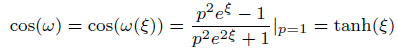              (8)

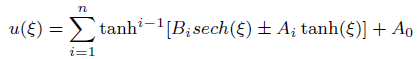
Where P is the constant of integral. These two significant solutions achieve the definition of the SGEM to get the solution of the NPDE of the form

              (9)

Now, we consider

              (10)

Now, due to equation 7 and equation 8, equation 10 can be rewritten as follows:

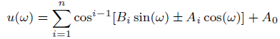              (11)

The value of n is obtained by balancing the highest power of nonlinear term and the highest derivative appearing in the transformed NODE.

Applications

The Space-Time Fractional STO Equation

Consider the space-time fractional order STO equation

              (12)

Using the transformation

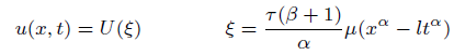              (13)

12 can be changed into an ODE equation

              (14)

Where

We get M = 1 as a result of balancing terms U ²U′ and U’’’ in 14 the solution can therefore, expressed as

              (15)

Where A0, A1, B1 are constant to be computed.

Description of Sine-Gordon Expansion method [17], will yield the following system of algebraic equations

              (16)

              (17)

              (18)

              (19)

              (20)

              (21)

              (22)

              (23)

case 01

              (24)

case 02

              (25)

case 03

              (26)

case 04

              (27)

case 05

              (28)

case 06

              (29)

case 07

              (30)

case 08

              (31)

case 09

              (32)

Solution1 (corresponding to case 01) (Figure 1)

Figure 1: Solution of (33) κ = 0.6, μ = 0.5, β = 2, A₀ = 0.05.

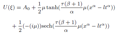              (33)

Solution2 (corresponding to case 02)

              (34)

Solution3 (corresponding to case 03)

              (35)

Solution4 (corresponding to case 04) (Figures 2-10)

              (36)

Figure 2: Solution of (33) κ = 0.6, μ = 0.5, β = 2, A₀ = 0.05.

Figure 3: Solution of (33) κ = 0.6, μ = 0.5, β = 2, A₀ = 0.05.

Figure 4: Solution of (33) κ = 0.6, μ = 0.5, β = 2, A₀ = 0.05.

Figure 5: Solution of (33) κ = 0.6, μ = 0.5, β = 2, A₀ = 0.05

Figure 6: Solution of (34) when κ = 0.6, μ = 0.5, β = 2, A₀ = 0.05.

Figure 7: Solution of (34) when κ = 0.6, μ = 0.5, β = 2, A₀ = 0.05.

Figure 8: Solution of (34) when κ = 0.6, μ = 0.5, β = 2, A₀ = 0.05.

Figure 9: Solution of (34) when κ = 0.6, μ = 0.5, β = 2, A₀ = 0.05.

Figure 10: Solution of (41) κ = 0.6, μ = 0.5, β = 2, A₀ = 0.05.

Solution5 (corresponding to case 05)

              (37)

Solution6 (corresponding to case 06)

              (38)

Solution7 (corresponding to case 07)

              (39)

Solution8 (corresponding to case 08)

              (40)

Solution9 (corresponding to case 09) (Figures 11-14)

Figure 11: Solution of (41) κ = 0.6, μ = 0.5, β = 2, A₀ = 0.05.

Figure 12: Solution of (41) κ = 0.6, μ = 0.5, β = 2, A₀ = 0.05.

Figure 13: Solution of (41) κ = 0.6, μ = 0.5, β = 2, A₀ = 0.05.

Figure 14: Solution of (41) κ = 0.6, μ = 0.5, β = 2, A₀ = 0.05.

              (41)

Space-Time Fractional Kdv-ZK Equation by Sine-Gordon Expansion Method

Consider the space-time fractional Kdv-ZK equation [19]

              (42)

And the transformation

              (43)

Where κ is nonzero constant, which on substituting in 42 give us the following ODE

              (44)

The trial solutions of (44) can be expressed as

U(𝜉) = tanh(𝜉) (A₂ tanh(𝜉) + B₂sech(𝜉))+A₁ tanh(𝜉)+A₀+B₁sech(𝜉)UsingEqs(??)intoEqs(44)theAlgebraicequationscanbewrittenas -aA₀B₁ aA²₁ +

              (45)

              (46)

              (47)

              (48)

              (49)

              (50)

case 01

              (51)

case 02

              (52)

case 03

              (53)

Solution corresponding to case 01

              (54)

Solution corresponding to case 02

              (55)

Solution corresponding to case 03

              (56)

Conclusion

By applying a complex wave transformation, we have be successful to obtain the solitons of the metamaterials with anti-cubic law of non-linearity. We have discussed the optical soliton solutions, along with some constrained conditions on parameters, of the metamaterials with anti-cubic law of nonlinearity via the modi_ed tanh expansion method. Many new optical solitary and periodic solitary wave solutions have been retrieved with the above afore mentioned integration scheme. These solutions are thus very encouraging to carry out future studies in this area.

REFERENCES

1. Podlubny I. Fractional differential equations: an introduction to fractional derivatives, fractional differential equations, to methods of their solution and some of their applications. Elsevier 1998; 27.
2. Inan IE, Ugurlu Y, Bulut H. Auto-Bäcklund transformation for some nonlinear partial differential equation. Optik. 2016;127(22):10780-5.
3. Wazwaz AM. Multiple-soliton solutions for the KP equation by Hirota’s bilinear method and by the tanh–coth method. Appl Math Comput 2007;190(1):633-40.
4. Zayed EM, Alurrfi KA. A new Jacobi elliptic function expansion method for solving a nonlinear PDE describing the nonlinear low-pass electrical lines. Chaos Soliton Fract 2015;78:148-55.
5. Naher H, Abdullah FA, Mohyud-Din ST. Extended generalized Riccati equation mapping method for the fifth-order Sawada-Kotera equation. AIP Advances 2013;3(5):052104.
6. Sakar MG, Ergören H. Alternative variational iteration method for solving the time-fractional Fornberg–Whitham equation. Appl Math Model 2015;39(14):3972-9.
7. Abdou MA, Soliman AA. New applications of variational iteration method. Physica D: Nonlinear Phenomena. 2005;211(1-2):1-8.
8. Soliman AA. The modified extended direct algebraic method for solving nonlinear partial differential equations. Int J Sci 2008;6(2):136- 44
9. Elwakil SA, El-Labany SK, Zahran MA, Sabry R. Modified extended tanh-function method for solving nonlinear partial differential equations. Physics Letters A 2002;299(2-3):179-88.
10. Zhang S, Xia T. An improved generalized F-expansion method and its application to the (2+ 1) -dimensional KdV equations. Commun Nonlinear Sci Numer Simul 2008;13(7):1294-301.
11. Navickas Z, Ragulskis M, Listopadskis N, Telksnys T. Comments on “Soliton solutions to fractional-order nonlinear differential equations based on the exp-function method”. Optik 2017; 223-231.
12. Navickas Z, Telksnys T, Ragulskis M. Comments on “The exp-function method and generalized solitary solutions”. Comput Math with Appl 2015;69(8):798-803.
13. Manafian J, Lakestani M. Application of tan (ϕ/2)-expansion method for solving the Biswas–Milovic equation for Kerr law nonlinearity. Optik 2016;127(4):2040-54.
14. Akbulut A, Kaplan M, Tascan F. The investigation of exact solutions of nonlinear partial differential equations by using exp (−Φ (ξ)) method. Optik 2017;132:382-7.
15. Li ZB, He JH. Fractional complex transform for fractional differential equations. Math Comput Appl 2010;15(5):970-3.
16. Wen-An L, Hao C, Guo-Cai Z. The (ω/g)-expansion method and its application to Vakhnenko equation. Chinese Physics B 2009;18(2):400.
17. Zhang Y. Solving STO and KD equations with modified Riemann– Liouville derivative using improved $(G’/G) $-expansion function method. IAENG Int J Appl Math 2015;45(1):16-22.
18. Kilbas AA, Srivastava HM, Trujillo JJ. Theory and applications of fractional differential equations. Elsevier, UK. 2006.
19. Kadem A, Kılıçman A. Note on transport equation and fractional Sumudu transform. Comput Math with Appl 2011;62(8):2995-3003.
20. Gao GH, Sun ZZ, Zhang YN. A finite difference scheme for fractional sub-diffusion equations on an unbounded domain using artificial boundary conditions. J Comput Phys 2012;231(7):2865-79.
21. Afzal I. Stationary Solutions and Optical Solitons for Nonlinear Schrodinger Equations (Doctoral dissertation, Department of Mathematics, COMSATS University Islamabad, Lahore campus).
22. Ekici M, Mirzazadeh M, Sonmezoglu A, Ullah MZ, Asma M, Zhou Q, Moshokoa SP, Biswas A, Belic M. Dispersive optical solitons with Schrödinger–Hirota equation by extended trial equation method. Optik 2017;136:451-61.
23. Naher H, Abdullah FA. Some New Traveling Wave Solutions of the Nonlinear Reaction Diffusion Equation by Using the Improved (G′/G)- Expansion Method. Math Probl Eng 2012.
24. Bulut H, Sulaiman TA, Baskonus HM, Aktürk T. On the bright and singular optical solitons to the ($ $2+ 1$$2+ 1)-dimensional NLS and the Hirota equations. Opt Quantum Electron 2018;50(3):1-2.
25. Zhang Y. Solving STO and KD equations with modified Riemann– Liouville derivative using improved $(G’/G) $-expansion function method. IAENG Int J Appl Math 2015;45(1):16-22.
26. Kaur L, WazwazAM. Bright–dark optical solitons for Schrödinger- Hirota equation with variable coefficients. Optik 2019; 179:479-84.
27. Yaşar E, Yıldırım Y, Zhou Q, Moshokoa SP, Ullah MZ, Triki H, Biswas A, Belic M. Perturbed dark and singular optical solitons in polarization preserving fibers by modified simple equation method. Superlattices Microstruct 2017;111:487-98.
28. Zhou Q, Ekici M, Sonmezoglu A, Mirzazadeh M. Optical solitons with Biswas–Milovic equation by extended G′/G-expansion method. Optik 2016;127(16):6277-90.
29. Zhou Q, Ekici M, Sonmezoglu A, Mirzazadeh M, Eslami M. Optical solitons with Biswas–Milovic equation by extended trial equation method. Nonlinear Dynamics. 2016;84(4):1883-900.
30. Hassaballa AA, Elzaki TM. Applications of the improved G/G expansion method for solve Burgers-Fisher equation. J Comput Theor Nanosci 2017;14(10):4664-8.
31. Khalil R, Al Horani M, Yousef A, Sababheh M. A new definition of fractional derivative. J Comput Appl Math 2014;264:65-70.
32. Sulaiman TA, Bulut H, Baskonus HM. Optical solitons to the fractional perturbed NLSE in nano-fibers. Discrete Contin Dyn Syst - S. 2020;13(3):925.
33. Ray SS. Dispersive optical solitons of time-fractional Schrödinger– Hirota equation in nonlinear optical fibers.Physica A: Statistical Mechanics and Its Applications.2020;537:122619.
34. Sardar A, Ali K, Rizvi ST, Younis M, Zhou Q, Zerrad E, Biswas A, Bhrawy A. Dispersive optical solitons in nanofibers with Schrödinger- Hirota equation. J Nanoelectron Optoelectron 2016;11(3):382-7.
35. Sardar A, Ali K, Rizvi ST, Younis M, Zhou Q, Zerrad E, Biswas A, Bhrawy A. Dispersive optical solitons in nanofibers with Schrödinger- Hirota equation. J Nanoelectron Optoelectron 2016;11(3):382-7.
36. Mohamad-Jawad AJ. The Sine-Cosine Function Method for Exact Solutions of Nonlinear Partial Differential Equations. ARUC. 2013(32):124-43.
37. Kilic B. Improved šG 0/GŽ-Expansion Method for the Time-Fractional Biological Population Model and Cahn–Hilliard Equation. J Comput Nonlinear Dyn 2015;10:051016-1.
38. Zuo JM. Application of the extended G′ G-expansion method to solve the Pochhammer–Chree equations. Appl Math Comput 2010;217(1):376-83.
39. Zuo JM. Application of the extended G′ G-expansion method to solve the Pochhammer–Chree equations. Appl Math Comput 2010 ;217(1):376-83.
40. Jumarie G. Table of some basic fractional calculus formulae derived from a modified Riemann–Liouville derivative for non-differentiable functions. Appl Math Lett 2009;22(3):378-85.
41. He JH, Li ZB. Converting fractional differential equations into partial differential equations. Thermal Sci 2012;16(2):331-4
42. Bulut H, Sulaiman TA, Baskonus HM, Rezazadeh H, Eslami M, Mirzazadeh M. Optical solitons and other solutions to the conformable space–time fractional Fokas–Lenells equation. Optik 2018;172:20-7.
43. Ismael HF, Bulut H, Baskonus HM. Optical soliton solutions to the Fokas–Lenells equation via sine-Gordon expansion method and $$(m+ ({G’}/{G})) $$(m+ (G′/G))-expansion method. Pramana 2020;94(1):1-9.
44. Cattani C, Sulaiman TA, Baskonus HM, Bulut H. On the soliton solutions to the Nizhnik-Novikov-Veselov and the Drinfel’d-Sokolov systems. Opt Quantum Elec 2018;50(3):1-1.
45. Gao W, Ghanbari B, Günerhan H, Baskonus HM. Some mixed trigonometric complex soliton solutions to the perturbed nonlinear Schrödinger equation. Mod Phys Lett B 2020;34(03):2050034.
46. Zhu SD. The generalizing Riccati equation mapping method in nonlinear evolution equation: application to (2+ 1)-dimensional Boiti– Leon–Pempinelle equation. Chaos Soliton Fract 2008;37(5):1335-42.