Time Blast Wave Theory for the Expansion of the Universe

Received: 25-Jul-2022, Manuscript No. PULJMAP-22-5199; Editor assigned: 27-Jul-2022, Pre QC No. PULJMAP-22-5199(PQ); Accepted Date: Aug 03, 2022; Reviewed: 29-Jul-2022 QC No. PULJMAP-22-5199(Q); Revised: 29-Jul-2022, Manuscript No. PULJMAP-22-5199(R); Published: 20-Aug-2022, DOI: 10.37532/puljmap.2022 .6(4); 01-12.

Citation: Jarvis G. Time blast wave theory for the expansion of the universe. J Mod Appl Phys.2022; 6(4):1-17.

This open-access article is distributed under the terms of the Creative Commons Attribution Non-Commercial License (CC BY-NC) (http://creativecommons.org/licenses/by-nc/4.0/), which permits reuse, distribution and reproduction of the article, provided that the original work is properly cited and the reuse is restricted to noncommercial purposes. For commercial reuse, contact reprints@pulsus.com

Abstract

A new theory is presented and tested that time itself is the phenomenon that causes the expansion of the universe and that without expansion, time would simply not be. The model of the theory accurately matches observed cosmological luminosity data consequently accurately describing the observed expansion of the universe. The theory implies that the universe exploded outwards within the dimension of time with all particles expanding from this event within a time blast sphere. Each space dimension is wrapped around the time dimension and every object that is gravitationally separate within the time blast-wave will progress on their own time trajectory of time away from time zero. This has the effect that all objects will expand or move apart as the time sphere expands. We observe distant, and therefore historic, objects on a spiral timeline. We have modelled the theory and shown strong agreement with luminosity observations both at low and high redshift without the need for a cosmological constant thus indicating that the universe is not accelerating in its expansion. The model in fact predicts it is decelerating. The theory also predicts that the unperturbed speed of time expansion will impose a limit on the universe in terms of the fastest speed possible and the speed that light must always travel at. With this limit and as no object can ever be stationary in the time dimension, but that faster and heavier objects will expand less, the theory consequently leads us to explain why special and general relativity occur. Gravity can be explained by the clumping of matter into the dimension of time causing a localised slowing of expansion subsequently causing time dilation and thus resulting in an attractive force with other objects. By this theory, black holes are not singularities but are simply dimples on the time blast wave front. The reason for wave-particle duality of tiny particles and photons is also explained by the finite size of the window over which we can perceive timeA new theory is presented and tested that time itself is the phenomenon that causes the expansion of the universe and that without expansion, time would simply not be. The model of the theory accurately matches observed cosmological luminosity data consequently accurately describing the observed expansion of the universe. The theory implies that the universe exploded outwards within the dimension of time with all particles expanding from this event within a time blast sphere. Each space dimension is wrapped around the time dimension and every object that is gravitationally separate within the time blast-wave will progress on their own time trajectory of time away from time zero. This has the effect that all objects will expand or move apart as the time sphere expands. We observe distant, and therefore historic, objects on a spiral timeline. We have modelled the theory and shown strong agreement with luminosity observations both at low and high redshift without the need for a cosmological constant thus indicating that the universe is not accelerating in its expansion. The model in fact predicts it is decelerating. The theory also predicts that the unperturbed speed of time expansion will impose a limit on the universe in terms of the fastest speed possible and the speed that light must always travel at. With this limit and as no object can ever be stationary in the time dimension, but that faster and heavier objects will expand less, the theory consequently leads us to explain why special and general relativity occur. Gravity can be explained by the clumping of matter into the dimension of time causing a localised slowing of expansion subsequently causing time dilation and thus resulting in an attractive force with other objects. By this theory, black holes are not singularities but are simply dimples on the time blast wave front. The reason for wave-particle duality of tiny particles and photons is also explained by the finite size of the window over which we can perceive time

Keywords

Astronomy; Theoretical physics; Universe expansion; Gravity; Black holes; Wave-particle duality; relativity; Time dimension

Introduction

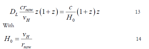
It is now generally accepted that the observable universe is expanding. This expansion was first experimentally measured by Hubble and can be expressed as the rate of expansion between two points in space as

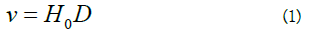
With H0 being the Hubble constant, D being the “proper distance” which can change over time and v being the recessional velocity[1]. The Hubble constant is usually quoted in km/s/Mpc and gives the speed of expansion of the distance between two astronomical objects 1Mpc apart. It is generally accepted that the Hubble constant has varied with time and today what it generally means is the current expansion rate. Roughly the current Hubble constant is generally thought to be about 70 km/s/Mpc. This means that it takes around a billion years for the universe to grow by 7%.

The above is usually explained as being an expansion in the metric of space rather than an expansion in space itself. Here we choose to look deeper at what this means and propose that it is the time dimension that is the metric of expansion and not some other completely hidden dimension. Einstein and others already proposed that time and space are intrinsically linked into a space time continuum and here we expand on that idea to propose a new theory that the big bang was not only the start of our universe but the reason why time exists[2]. What we propose here is that the “big bang” event that is believed to have occurred 13.8 billion years ago should be thought of as a time zero event – a point in time in which the objects of our observable universe started out on their journey through what we conceive of as time [3]. Time can be thought of as another spatial dimension, one for which only a small sliver – a thin peel of a sphere – is observable at any instant. Every gravitationally distinct object that was caught in this time explosion is expanding outwards on its own trajectory away from time zero on a time blast sphere. We have tested this theory by modelling it and comparing to the available observations to prove that such a theory is not only plausible but explains why the cosmos is fundamentally limited by the speed of light and gravity behaves the way it does. Finally we look on a particle level, and explore how this concept can explain wave-particle duality.

Historically, many techniques have been used to measure the Hubble constant to varying degrees of accuracy. Direct measurement can be performed using parallax techniques on nearby Cepheid variables. They can then be used to calibrate them as known “candles” which give out a predictable amount of luminosity so that distances to Cepheids in nearby galaxies can be measured. Type 1a supernovae which flare much brighter can then be used, calibrated against nearby Cepheids, to go further into space beyond the limit of the Cepheid variables. The observed red shift of the light received then gives the speed of expansion for the different distances. This type of technique is called a distance ladder technique. Generally, for redshifts<0.1, a linear relationship of expansion is observed[4].Using purely the photometry of Cepheid variables in the Large Magellanic Cloud, which is 0.05 Mpc away from the earth, then perhaps the most accurate value from direct parallax measurements for the Hubble constant to date of 74.03 ± 1.424 has been obtained. These measurements are model independent and give a picture of the late universe how it is expanding now. Such techniques have been used up to a redshift of 0.4 where the Hubble constant has been measured to be 73.24 ± 1.74 km/s/Mpc and show a strong linear relationship of expansion with distance over this region[5]. By contrast modelled Cosmic Microwave Background (CMB) data suggests an expansion rate of 67.66 ± 0.42 km/s/Mpc[6]. The cosmic microwave background is believed to have originated at the point during expansion when the energy density became favourable for electrons to combine with protons to form hydrogen. This is thought to have happened when the universe was about 380,000 years so this data can be used to extrapolate from this early image to the expansion rate we see today[7]. There are many other techniques that have been employed, but whose uncertainties are perhaps not small enough to be conclusive about any further differences[8]. However, as can be seen, there is discrepancy between the two main techniques which do not agree within their error bars.

Further to the above controversy, there is significant evidence obtained from type 1a supernovae luminosity data at higher redshift (>0.3) that the universe might still be accelerating as luminosities appear to be on average 10% -15% dimmer (and thus further away) according to current models than they should be in a universe that were not accelerating in its expansion. Other more detailed studies have subsequently supported these findings[9,10].

We start by describing how the time blast wave model can describe a universe that is expanding in a roughly linear fashion in recent times. We then address the possible accelerating universe as we model against the observed luminosity data.

Theory Explained

Simply put, the theory is that time is a spatial dimension, which obeys the same laws of physics as other space dimensions but is largely invisible to us. It is only visible as an expansion effect in the 3 spatial dimensions we can observe and results in us experiencing time. This is shown in Figure 1 with the small sphere representing 3-dimensional space which is being expanded along the blue lines by time. Time does not progress in a single direction, but in all directions at once creating a spherical universe. Another way of putting this is that time is the same as space – there are 4 dimensions of space- but we travel, “in time” along one of them.

As it is difficult to describe more than 3 spatial dimensions at once, then if we imagine we are looking only in one plane where 2 dimensions can be viewed – one normal space dimension and the dimension of time. Imagine a cross section through the centre of the spheres as indicated by the orange patching in Figure 1.

Figure 1: Visualization of the dimension of time signified by the blue lines causing the expansion of 3D space. Orange patching shows a cross section through a single space dimension as described further in Figure 2

Time will progress outwards as shown in Figure 2, away from the origin (zero volume sphere in Figure 1) along the radius with the space dimension signified by the circumference continually expanding as the radius (time) increases.

Figure 2: Visualization of Time blast wave cross section cutting through a single time dimension (as shown by the radius) and a single space dimension (as shown by the circumference). This blast wave started at time t0 and has reached time t1. Two gravitationally distinct objects are shown revealing how they would expand away from each other in space as the time blast wave increases. The thin black line shows the observable slice of time with the grey areas showing the possibility of matter existing outside of our observable time window.

Observers present in the space dimension will have a view across the circumference yet only be able to appreciate a small sliver of the dimension of time as signified by the black band in the figure. The bands of grey show the possibility that matter within the time blast wave may be present yet hidden within a preceding and subsequent part of the time blast. An initial explosive burst of force would propel all objects in the universe away from time zero. If the time dimension behaves as a frictionless vacuum, then once up to speed they would then on average progress in the direction in which they were propelled at a constant speed. The significance of this is that all gravitationally distinct objects would propel outwards, and this would then reveal itself in the visible space dimensions as an expansion effect.

The circumference of the blast wave has a linear relationship with regards to the rate of increase of radius of the time blast sphere, r. At any point in time, the rate of increase can be said to be:

(Note this is independent of acceleration).

An arc of the circle with angle σ (in radians) and of length C would be increasing by

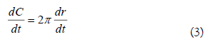
This basically says that as the radius increases, then an arc defined by a certain angle will also increase linearly with time. Therefore, if each object in space has its own timeline emanating from time zero, it will appear in a spatial sense to move away from other objects at different points in the circumference of the blast wave without the need for another force (other than the initial explosive force that kicked off the time expansion in the first place).

The time blast sphere expansion model can therefore explain qualitatively at least a universe that is increasing locally in a manner consistent with the simple Hubble rate shown in equation 1. To test the theory further though, we need to expand this to model out further to more distant objects whose expansion has been measured by variations in luminosities. We therefore need to consider what would be the impact on the luminosity of objects as we investigate to larger distances.

Impact on observations of distant objects in the universe

As light reaches us from distant objects across the universe, we will be witnessing prior incarnations of objects whose luminosity has diminished by the distance that the light has travelled.

If we take a slice through time and a single space dimension as before and plot the radius of the universe as it was when the light that reaches us was emitted versus its radial distance from us, we will end up with a spiral as shown in Figure 3.

Figure 3: Visualization of the spiral effect of a time blast expanding universe caused by the speed of light having a fixed value. Scale for both x and y is in Mpc. Distant, and therefore historic, objects in the universe, if observed from point A will appear as if on a spiral path reaching back to time zero.

Note that the observer sitting at A would not appreciate the curvature as the curvature would purely be within the time dimension – so in spatial terms it would look “flat”. Also note that this effect would be duplicated in the other two space dimensions. However, as a single light beam would effectively be operating over this single space dimension (it has little in the way of height or width) then this model should accurately portray a single pinpoint light source reaching us at the Earth and allow us to model its effects accordingly. This is basically saying we are aligning the path of our photon beam up with an arbitrary set of x, y, z axes that is consistent with our cross section of time/space. A different photon would require a different cross section/alignment, but the spiral path would simplify to be the same and be dependent only on the distance to the object being observed.

The spiral effect would be created because the light that travels along the circumference of space will always travel at the same velocity. As it takes a finite time for light to travel from one point to another, then by the time light reaches a second object, the space dimension has already increased in size due to the increase in radius of the time blast sphere. In Figure 3 the radius at point B is slightly smaller than the radius at point A. As you travel further back in time, the effect is greater. Basically, for the same distance that light travels, the angle of the spiral would increase the more distant (historic) the light is and the spiralling effect as shown in the Figure 3 would be observed.

Resultant Impact on luminosity

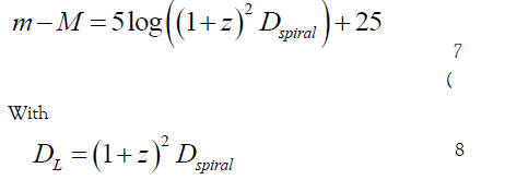
The magnitude of observed light (expressed as a distance modulus m-M) of any object is related to the luminosity distance by

where D_L is the luminosity distance in Mpc and can be defined as

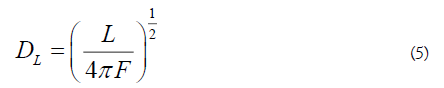
L is the intrinsic luminosity of the object and F is the observed flux. For nearby objects (ones for which the time that has passed is minimal and there has been little increase in radius) this would approximate to the distance around an arc of our spiral model, Dspiral. For objects that are further away, then this will be distorted. If a light “packet” were travelling from one object to another around the spiral path, then the increase in circumference of the time blast would cause a stretching of the light wave. This expansion would show up as redshift, the deviation in wavelength between the emitted and observed light. This stretching would consequently cause a dimming effect on the magnitude of the light observed by two mechanisms:

• As the light stretches, then the energy of light will diminish which will cause a reduction in intensity. The wavelength of light will increase relative to r_now /r_then as the circumference now is proportionally bigger for the same angle, so consequently the energy of the light will drop in intensity relative to r _then /r_now.

• Secondly the stretch will mean that the photon arrival rate within a beam of photons would be reduced again according to r_then/r_now.

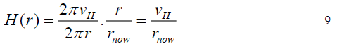
The redshift observed for any point around the spiral should be directly related to the size of the universe at that point i.e., the circumference. As the circumference of our blast sphere is directly proportional to the radius, then the stretching effect or redshift

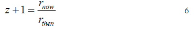
where z is the observed redshifti. So, for any point in our modelled spiral, we can calculate the expected redshift. The total distortion effect expected due to the increase in universe size would be 1/(1+z)2. We therefore need to do the reverse and apply this factor to our distance to get the right luminosity modulus that should be observed:

Calculating the expected recessional velocity

The velocity of expansion can be calculated between any two points on the light spiral by calculating the angle between them and the distance light would take to travel across the arc and comparing this to the circumference of the circle at that point in “time”.

As noted above, the angle increases for the same distance travelled as you head back in time, so if this were the only effect, then a distortion in the velocity observed would occur with the apparent rate of expansion increasing as you looked to more distant objects. In other words, even if you had a constant rate of increase in r, the rate of expansion would appear distorted as we would not be looking at the true distance around a circular arc but rather at a distance around a spiral arc. The rate of increase of the circumference can be seen in equation 3. To obtain the true rate of increase we would need to multiply this velocity obtained by ½ πr with r in Mpc to get the amount of total circumference that accounts for 1Mpc.

However, there is also a contrary distortion effect of the light that we observe that is caused by the fact that light from B would take so long to reach A it would be reflecting a younger version of B which consequently would have had less time to expand, meaning that it will appear as if it is separating to a lesser extent than if the objects were at effectively the same point in “time”. In other words, the radius of the historic object would be less. This turns out to have the exact opposite distortion i.e., r/rnow.

So, mathematically both these distortion effects cancel each other out so that a linear relationship relative to r would still be observed versus the distance from Earth, even though the light would reach us from a spiral arc path. So, the expansion rate is

where vH is the observed rate of increase in r or resultant velocity of timeii (with any internal interactions included). The spiral distance of a light beam’s origin to earth can be seen to be the integral of the light travel distance:

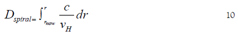
And Luminosity distance can therefore be calculated, allowing for dimming effects discussed above by:

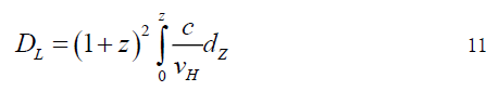
where c is the speed of light.

If we assume, to start with at least, that the rate of expansion is constant i.e., vH is a constant, independent of r then

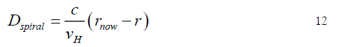
Combining 7, 8 and 9 reveals

Fitting observations to our model

As well as fitting to the observed luminosities we want to ensure that we broadly constrain ourselves with other studies regarding the known “current” Hubble expansion rate, H0. As stated in the introduction the best measurement for the expansion rate as observed locally – our best estimate for the rate of expansion now – can be taken from the direct parallax measurements of nearby Cepheids 74.03 ± 1.424. The figure obtained by CMB is 67.66 ± 0.42 km/s/Mpc6. Our model should therefore predict a figure that falls within these two extremes for it to be valid.

Estimate for the “Speed” of time

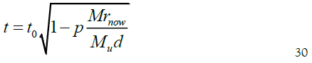
These measurements allow us to derive an estimate for the current “speed” of time – the rate of increase in the radius of the blast sphere and to then use it to check that the model produces a consistent “speed”. Assuming time expansion is roughly constant away from time zero at our current point in “time”, this would mean that time is basically the distance we have travelled in the dimension of time (radius of expansion) for a constant expansion velocity:

From the above we can estimate the expansion velocity – the expansion that we experience purely as time. We can work backwards from the Hubble constant to figure out what the current time expansion velocity is.

Taking two points in the universe 1MPc (3.086 x 1022 m) apart it would take light 3.26 million years (1.02938 x 1014 seconds) for light to travel between them.

Taking the expansion rate of these two points to be 74.03 km/s as stated above, then during this time the objects distance apart would have expanded by:

74030 x 1.02938 x 1014 m =7.62049 x 1018 m.

The original distance of the objects before the light beam left would have therefore been:

3.0860 x 1022 - 7. 62049x 1018 = 3.08524 x 1022 m.

As an approximation then using Pythagoras theorem this would mean that the radial expansion in the dimension of time would be 6.858 x 1020 m. From the “distance” and “time”, we can then calculate the speed of expansion to be:

6.662 x 106 ms-1 = 0.022c, where c is the speed of light.

If we take the expansion rate of these two points to be 67.66 km/s (as per CMB data calculations) as stated above, then the speed of expansion would be:

6.369 x 106 ms-1 = 0.021c, where c is the speed of light

If we take the expansion rate of these two points to be 67.66 km/s (as per CMB data calculations) as stated above, then the speed of expansion would be:

6.369 x 106 ms-1 = 0.021c, where c is the speed of light.

All the above can be applied to model against the observed data. Once the above has been modelled, we can then compare luminosities of observed astronomical objects to see if the time blast sphere model which would result in a spiralised light path ties in with observed luminosities of objects in the universe.

Comparison with observed luminosities

Using equation 11 combined with the distances from the above spiral path we can predict the luminosities that would be observed at different distances as observed from Earth if v_H were constant.

The predicted magnitude observed versus z with a constant value of vH can be seen as the orange dotted line in Figure 4 and 5. The fit shown was obtained using a v_H = 6.714 x 106 ms-1 with a current day time, radius of 95.03 Mpc which equates to a Hubble constant of 70.65 km/s.

Also shown for comparison we have shown the observed set of type Ia supernovae luminosities as used by Reiss et al. (1998) and Betoule et al (2014). [11]Reis et al (1998) and Betoule et al (2014) took care to fit light curves and calibrate against the low z data to give an accurate picture of the true luminosity moduli. As can be seen, a reasonable fit is obtained at low z (close the earth) but at larger z a larger modulus (less bright) is predicted than is observed. This suggests that historically the rate of expansion was greater, and that the universe is currently decelerating.

If we let the speed of expansion vary over time by fitting the data to an exponential decay functioniii, then we can obtain good correlation with the observed data as shown by the red solid line.

Figure 6 shows the varying value for vH expressed as a faction of the speed of light versus z which was produced in creating the solid red line fit shown in Figures 4 and 5.

Figure 4: Best fit modelled time blast wave allowing a fixed speed of expansion (orange solid line) and a varying speed of expansion (red solid line) versus observational data taken by Reiss et al. (1998) and Betoule et al (2014) (points).

Figure 5: Same data as Figure 4 but with z shown on a logarithmic scale.

Figure 6: Variation of the speed of expansion as a fraction of c versus z that produces the best fit to the luminosity data

The other results of the fit to the data can be seen below

• Effective velocity of time today, vH= 0.0219c or 6556.9 km/s

• Current Universe Blast Sphere Radius= 95.02 Mpc

• Current Circumference of Universal Blast Sphere = 597.1 Mpc

• Total distance along spiral light path to time zero= 3248 Mpc

• Hubble constant of 68.98 km/s

As can be seen, the model proves that the theory of a universe expanding in the dimension in time and allowing the acceleration/retardation to vary over time (governed by an exponential decay to model the deceleration of the blast wave) can accurately predict the luminosity observations and predict an expansion rate consistent with previous determinations. The model also predicts that the speed of expansion is slowing. This is perhaps not a surprise as the idea of uninterrupted expansion perhaps seems unrealistic for several reasons. For one, the interactions of the objects of the universe themselves are likely to cause a retardation and this retardation as time goes on will decrease as objects move further away. Also, the energy of the explosive blast might not be entirely focussed to a single instant but rather might transfer between the objects of the early universe to only later be released as kinetic energy. However, the above is in direct contradiction with the conclusions using the Friedman equation and discussed by Reiss et al (1998) who determined that the rate of expansion is currently increasing. This will be discussed later in this paper.

The light spiral from our best fit can be seen in Figure 7. The shape of the spiral beyond the second orange dot moving from the outside in is dependent on the fitting equation picked. So, this part of the plot should be treated with caution and is shown here purely for interest. It is one possibility of the truth if time expansion did follow an exponential decay as described in Appendix 1 within the early universe. The points highlighted in the time spiral in Figure 7 are in order moving outwards from the centre, t0, location of most distance object so far observed (as of 2016) with a redshift of 11.0911, most distant data point from luminosity data and Earth.

Figure 7: Explanatory figure to illustrate the effects of movement on the resultant momentum vectors in a single time (vertical) and space (horizontal) direction. The case considered here is one of an object breaking up and being pushed apart creating two identical mass objects moving in opposing directions with the same velocity.

Again, note we are showing a single dimension of space and “time” and the light spiral of distance and radius which should be accurate for light travelling along a straight path. Obviously light will originate from different points and be on different spiral paths – every photon will have its own path, but it will follow the same type of spiral and can consequently be used without having to consider all dimensions at the same time Figure 8.

Figure 8: Explanatory figure to illustrate the effects of movement on the resultant momentum vectors in a single time (vertical) and space (horizontal) direction. The case considered here is one of an object breaking up and being pushed apart creating two identical mass objects moving in opposing directions with the same velocity.

The best fitting exponential decay model predicts that a constant velocity will eventually be reached of around 2% of the speed of light or 6.008 x 106 ms-1.

FURTHER DISCUSSIONS AND CONSEQUENCES

Time Dilation from Movement

Assuming no external effect is present, the slowing observed must mean that the interactions between the particles of the universe themselves is slowing the overall expansion rate. So how might this happen?

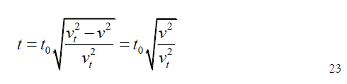
If an object is stationary in normal 3D space, then because of expansion it will move as described in previous sections away from time zero with a velocity which we might initially define as vt, the pure velocity of time. If we assume that the universe is a closed system with expansion occurring in a frictionless vacuum of time, then the momentum of the whole system must be conserved. If we consider a smaller closed system to start with that results in movement – a mass breaking apart equally for whatever reason (this might be a particle breaking apart or even two equal mass astronauts in space pushing away from each other) then the situation shown in Figure 9 would occur. Note to keep things simple we will initially set mA=mB and vA= vB. In the figure, the vertical direction signifies time expansion and the horizontal direction spatial momentum. The momentum in the horizontal direction is zero before “push off”. After “push off” then the overall momentum is still zero as the sum of the vectors of the two red arrows cancels each other out. However, as described in the previous section, the original particle is already moving in the time dimension so this momentum must also be conserved. As can be seen, the resultant momentum pA+pB must then equate to the initial momentum pt that comes about as a consequence of time expansion. As is clear, the resultant objects end up deviating on their path away from the origin of time. Let us assume to start with that the sum of the resultant masses are equal to the starting mass. If this were the case, then the resultant vector diagram would lead to:

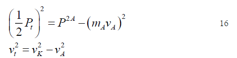
Figure 9: Explanatory figure to illustrate the effects of movement on the resultant velocity vectors in a single time (vertical) and space (horizontal) direction. The case considered here is one of an object moving sideways – half of the break up from Figure 9, for example.

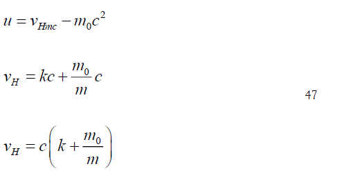
Where vt is the velocity of time, vA is the velocity of the particle in space and vX is the resultant velocity vector. But – where did the energy come from to generate the push off? If it was simply a translation of the kinetic energy, then this would lead to:

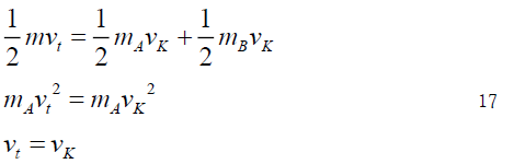
This clearly is not the case. Consequently, it must be the mass of the object, rather than the velocity that provided the energy and must therefore change when it splits apart, so

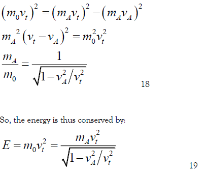
So, the energy is thus conserved by:

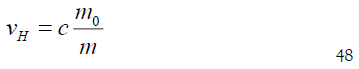
Where m0= ½m and m is the original non-moving (except in time) mass. In other words, our model suggests that the kinetic energy of expansion will reveal itself as mass if it deviates from its direction. The above means that if the universe is in spatial motion, then it will have a larger observable mass than if it were only moving in time. As we have deduced that the magnitude of the velocity in the time dimension does not change but instead the mass does, then the velocity vector diagram would look like that shown in Figure 9 comparing moving (blue) and non- moving (orange) particles. So as more and more particles interact and move, then the observed expansion velocity vres would end up being a lower value than the actual velocity of time. The relationship between the observed expansion velocity and the velocity of time is consequently:

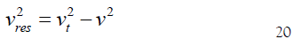
At velocities where v is a lot smaller than vt, then the overall velocity would be completely dominated by vt such that v is inconsequential. A value of v=0 gives us the non-time dilated limit or non-moving (apart from expansion). As soon as v approaches the value of vt then it will start to be important. At the point where it equals vt, then the velocity vector triangle would be a straight line, signifying this as the limit of speed which you could achieve in the universe.

On a universal level, then going from zero “sideways” motion to lots of “sideways” motion would have an overall effect. This is likely to have been greatest during the initial “explosive” phase. This effect over the whole universe would be:

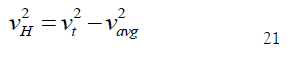
The velocity of expansion we measure, vH is really an averaged out effective velocity of time of the objects of the universe relative to the Earth.

Therefore

If we consider the inverse of the above situation – an object slowing down in space for some reason. This must mean that the object loses mass and therefore must gain velocity in the direction of time expansion to keep the momentum constant. So, this would drive the expansion of the universe up resulting in an overall equilibrium with mass/energy being passed back and forth into and out of the time dimension.

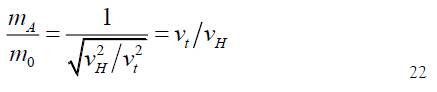
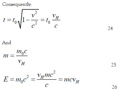
On the scale of individual objects, however, the dilation effect will still cause time to change dependent on how fast a particle is travelling relative to other objects that are moving differently. It will effectively create a dimple in the time expansion sphere. The effective time dilation observed would be as seen below:

The time blast sphere expansion theory therefore predicts that there will be a speed limit to the universe – that nothing in the universe is able to travel beyond a finite value, the un- impeded speed of time, vt. We have also shown that as particles move, their effective mass increases and time will dilate as a ratio of that maximum velocity.

As we know, there is a limit of speed to our observed universe and as it behaves in the same way as described above, then we conclude that the unimpeded speed of time vt must be equal to the speed of light, c. Conversely, we conclude that our universe has a speed limit because it is the speed at which time expansion would travel if nothing were there to slow it down.

If we return to Figure 9 and think about what happens if we were to go at the speed limit, c, we can see that this is essentially the same as returning to zero sideways movement – except the direction has changed - the sideways velocity would return to zero once again and the velocity in the time direction would equal c again. At this point, then the triangle becomes a straight line, and a dimension of space is lost. This would mean that it would appear to have zero volume and consequently zero measurable mass in 3D space. The photon may have mass, but it is hidden within the time dimension. This is discussed later but the important part for now is that once a particle reaches that limit it must turn into a photon (or split apart to become multiple photons), and can only progress across space at a speed limited to c. Our time model thus not only predicts that there is a speed limit on the universe but that if a photon were emitted from something, it would always travel at the speed of light.

In a sense, the emission of radiation can be viewed as the driver of expansion wherever it occurs and where it collides or is absorbed, then energy is turned into matter with a consequence that expansion is slowed. So, the continual absorption and emission of radiation will mean that the expansion on the photon level is bursting but on a universal level it will lead to isotropic expansion that appears to occur from every point in space.

If we take the ionisation of Hydrogen into a proton plus an electron by injecting a photon, this is similar to the model described qualitatively in above except that the two resultant particles are of different mass. This matters not to the overall mathematics if we take the total mass of the resultant proton and electron. We can calculate a resultant effective deflection velocity away from the direction of time from the (Mass of the Products – Mass of Reactants) by:

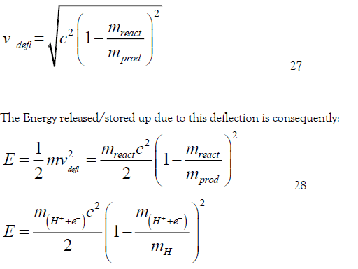
The Energy released/stored up due to this deflection is consequently:

The above calculates to be 13.59eV which is the ionisation energy of Hydrogen. This of course is the same as Einstein’s famous theory but we have reached it by a different means by treating time as a spatial dimension.

Everything is travelling at the speed of light in one of 4 dimensions. If it is travelling perpendicular to the time path – we see the object travelling at c and it appears as light. If it is travelling with the timeline, we will not observe it. Any distance in between and we observe the object to be travelling along our timeline and it will appear to have mass.

If we consider equation 27 in light of what this means – what deflection velocity would we end up with. Basically, as the mass of the reactants in 3 D space is zero (as we are talking about 2 photons) then this means that the deflection velocity must be zero – so we hit the scenario straight away with the creation of the first particles that they will be ejected perpendicular to the direction of expansion i.e. thrown into the 3D world at the speed of light. Which immediately suggests that these initial “particles” must also behave as photons, but the direction of travel has changed. This direction change is critical as at that point we would have a lot of photons that are going to collide head on or with glancing blows which will then allow resultant ejections to not be at right angles to the timeline and therefore be able to exist as mass.

Note the initial collision of light photons would have been unusual in another way as if all initial photons originally emanated from a single place and expanded from there then they would never have the opportunity to collide. However, as we believe that photons are spinning in time (see wave nature of light section) then it means that the initial photons would be able to collide with each other because of their spin.

Gravity

In the time expansion model, every distinct object in the universe has its own time trajectory within the time blast. As objects clump together and create a more massive single entity, then, by definition, they are not expanding away from each other as they coalesce. This moving towards each other will cause a time dilation (the universe expansion will be distorted) meaning that heavier objects will end up further back within the time blast wave. The more massive the object becomes because of this coalescence, the more dilated the time will therefore be in that area of space. In effect a dimple will be created in the time blast sphere wave front, slowing the time in this region of space, which will mean that any object passing will accelerate towards the clump. And those objects that have been accelerated towards the massive object will in turn add to the combined mass of the object. Where more clumping has taken place, these areas of the blast wave will sit closer to time zero than areas that have not clumped together.

In a sense you can view it like an energy scheme with more massive objects not necessarily moving slower but sitting further back in the time blast. If anything moves towards such a massive object, it will experience a slowing of time proportional to the object’s mass which will result in an acceleration towards the more massive object. The massive object would also “benefit” from the combination as once combined, the resultant object would sit even further back within the time blast. i.e., objects sit in a time dilation well within the time blast wave front attracting anything that comes near with a force relative to the object’s mass. The depth of the well would be proportional to the object’s mass.

Another way of thinking about it is that the mass of an object will be coalesced into a single time stream and that as time within that object is shared, it will have the same point-like trajectory as that of a single particle or photon. But the object must occupy “space” even within the dimension of time so in the time dimension the mass stacks linearly – a more massive object distorts the time blast wave by a larger extent compared to a smaller mass. It is possible since we believe all mass appears to have come from light that the stacking is related to the quanta of light with a single stacking unit being constrained to a fixed size by the photon it originated from. If it is quantized though, the stacking unit is so small that it appears continuous.

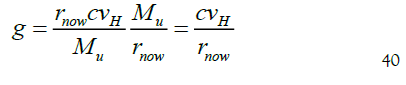
The depth of the dimple will be directly proportional to the mass of the combined objects (taking off the average mass at the blast wave front) relative to the mass of the universe Mu and must be some factor of the blast sphere radius. i.e.:

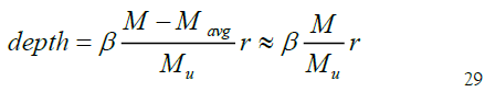
With being a dimensionless “constant” of proportionality between 0 and 1. This basically defines how much overall effect the retardation caused by “stacking” of mass within one timeline has. In cases where ��avg is small compared to M then this can be simplified as shown. If were 1 then coalescence of the whole universe would cause a dimple the size of r meaning that expansion would not occur.

From the above, we can therefore write an equation defining the time dilation caused by this dip in the front of the blast sphere. The time dilation effect in 3D space can be determined by also considering the 3D distance, d, of the object from the center of mass of M:

We can therefore say that the depth of the dimple would also define the Schwarzschild radius in 3D space, and we can relate the above to the universal gravitational constant by:

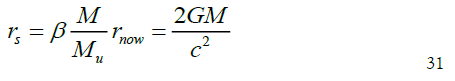
Where G is the gravitational constant. For G to remain constant as the universe expands then

must be inversely proportional to the only variable rnow.

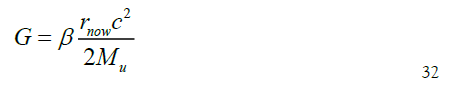
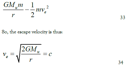
We can derive the above in a second way by returning to the section on the speed of light being the speed limit of the universe and to say that this is therefore the escape velocity of the universe – we know that c is the velocity of time if left unchecked so if it were possible to go beyond that, then light would escape the universe. Consequently, if we combine with Newton’s law of gravity and describe how a single mass m is attracted to the rest of the mass in the universe then:

From this, the Schwarzschild radius of the universe is:

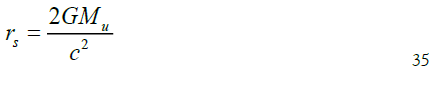
As we know that c is the limit of the universe, then rs=rnow and therefore:

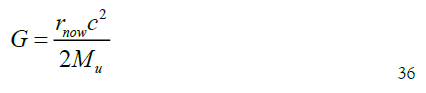
This would indicate that β from equation 28 is 1. However, since we are talking about the escape velocity being the speed of light, then equation 29 needs to take this into account and should therefore be

and should be thought of as the average ratio for all matter in the universe. The interesting thing here is that if the escape velocity of the universe is always c, then the time dilation of combined mass, gravity, will always balance off against this by this equation. Combining equation 25

The acceleration of a miniscule amount mass, towards the centre of the universe would be:

For a larger mass then the velocity of expansion will be reduced from vH by an amount relative to the ratio of the mass of the object to the mass of the whole universe and the effect will follow the inverse square law dependent on the 3D distance. Thus, the acceleration at the surface of the earth will be defined by:

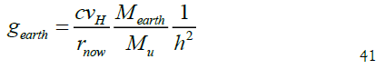
Where h is the radius of the earth. From this we can see that as the universe grows, the acceleration experienced by an object of a certain mass towards the centre of the universe will decrease. We can visualise this as an increase in the surface area of the time blast sphere’s wave front causing the dimples of combined mass to stretch out meaning that the side of each dimple is less steep thus decreasing the acceleration effect observed. Conversely, as G is proportional to rnow then the stretching of space means that when two objects do come closer together the time dilation experienced will be greater and the force experienced between them will therefore be greater. This will be caused by the fact that the depth of the gravity well is governed by depth of the gravity well is governed.

The above is the way gravity can be explained by the time blast sphere model.

Comparison with other models/studies

The hubble constant

In terms of the Hubble constant H0 we do have broad agreement with previous studies with a modelled current expansion rate of 68.98 km/s/Mpc. Betoule et al 201411 used 70 km/s/Mpc for their best fit to the data. We are unable to reconcile the higher values observed from local data such as the Magellanic cloud data of Reiss et al 20194 or Reiss et al 20165. Our best fit across the whole range of data modelled here would suggest a lower value.

We used the data presented in the Betoule et al 2014 study to model against as it was readily available and stretched to higher z compared with the later studies mentioned. Higher z although more intrinsically inaccurate due to its distance is likely to, by its very nature, have less emphasis on local movements i.e., objects may be moving apart by local movements unrelated to the overall expansion and these will be more apparent the closer you are to them. Basically, when we measure the redshift or blueshift of a galaxy, it will be the sum of the cosmological redshift and Doppler shift from the peculiar motion of the specific galaxy. If we look at the Andromeda galaxy (which is about 0.7 Mpc away) it is locally moving towards us at such a rate that it appears blue shifted so we know local effects are present[13].

Clearly it would be hard to distinguish positive local redshift effects from cosmological expansion. The studies cited here do discuss inhomogeneity of matter in the local universe but suggest it is negligible. But it is hard to rule out entirely that whole clusters of nearby galaxies might have their own motions that disrupt the Hubble expansion measurement and any ladder measurements that rely on them. These local effects will however be diluted as you look further and further away and include more variety in data points so although you can more accurately measure local phenomenon, a broader far-distance set of data is more likely to give a less distorted measure of H₀.

As both Betoule et al 2014 and Reiss et al 2019 and 2016 overlap for z<0.4 it is puzzling why both do not have more similar Hubble rates reported. The answer to this probably lies in the “calibration” of the distance ladder – the luminosity modulus data modelled against here was taken from the calculation as presented in Betoule et al 2014. However, the luminosity modulus is not a direct measurement but is itself derived from an equation that comes about due to how bright the objects are believed to be which is modelled. So, although the pattern of luminosity decrease may be accurate – the absolute value may be incorrect by a factor relating to the calibration of the luminosity data. The fact that we agree well with the study whose data was used supports that our theory can accurately predict the pattern of the universe’s expansion. If the data used is indeed off by a “calibration” factor, then our model would still be able to fit the data, but it would give a different Hubble rate dependent on this calibration.

The Friedman Equation

Figure 10 is a duplication of Figure 4 with other fits added in for comparison. As has already been discussed, the time blast wave model predicts that the universe expansion is currently decelerating. This is at odds with previous conclusions/models used.

Figure 10: Duplication of Figure 4 with addition of Friedman fits for Cosmological models ΩM=0.3, ΩΛ=0.7, ΩM=1 and ΩΛ=1 for comparison.

Just to emphasise, the model employed by us maps out the path a photon takes across space it will follow a simple spiral path in time (but flat in space). We have considered only one dimension of space and one dimension of expanding time as we have assumed that light travels in a “straight” line along the path. Although light will have obviously travelled through 3-dimensional space and each photon would follow its own path, each path would be straight and the time it takes to reach earth would purely depend on the distance along that single dimensional line. As the properties of light travelling through space are independent of the dimension it travels, this will mean we do not need to consider 3 dimensional effects in determining the redshift or relative luminosity in our model.

Reis et al (1998) and Betoule et al (2014) (and others before and since) used the Friedman equation to model the expansion of the universe and determine from this whether it is expanding or contracting. The Friedman equation tells us how the universe expansion varies with time based on the density of the universe and its curvature and was originally derived from Einstein’s field equations to be:

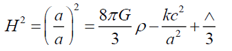
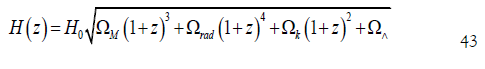
Where H is the time dependent Hubble constant, a is the scale factor of the universe relative to today, ρ is the density, G is the gravitational constant, and k is a constant and can be+1, 0 or 1. k defines the curvature of the cosmological model, with 0 signifying a flat universe. Density is believed to be made up of matter and radiation with the former decreasing in density by 1/a³ as you would expect from simple volumetric increase and the latter by 1/a⁴ the additional power being due to the stretching of light causing an additional decrease in energy. An additional parameter is also thought to be relevant Λ, called the cosmological constant that is believed to exist due to unseen “matter” called dark energy.

So, taking all this into account we can rewrite the red shift dependent

This basically says that the Hubble constant will change in time as revealed by a change in the redshift z. Ω= ΩM+ Ωrad+ ΩΛ=ρ/ ρcritical. ΩM is the mass density of the universe and ΩΛ is a re- writing of the cosmological constant and is responsible for acceleration or deceleration of the universe with ΩΛ= Λ/3H2. Ωrad and Ωk account for the relativistic mass and curvature,

respectively. Today’s consensus is that only 2 components are relevant as the radiation effect would have only been pertinent in the early universe and there is little curvature observed. Therefore, in the study by Reiss et al and Betoule et al, only a two-component model is used with ΩM and ΩΛ considered. The calculated luminosity distance in the Friedman model can then be calculated from this to be:

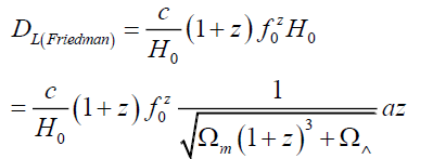
Three fits to this model are shown in Figure 11, one for the best ΩM=0.3, ΩΛ=0.7 (currently accepted values and close to those determined by Betoule et al – sometimes termed the concordance model) with H0=70 km/s/Mpc which agrees well with the data, one for ΩM=1 and one for ΩΛ=1. ΩM=1 is thought to describe a nonaccelerating model mentioned which predicts that the objects should be brighter than they currently are (lower modulus). As can be seen, the concordance model fits the observed data well like the decelerating time blast model. We also agree reasonably well with the resultant value of the current Hubble expansion rate.

However, the conclusions drawn from both models are inconsistent with each other. As the ΩM=1 sits below the ΩM of 0.3, ΩΛ of 0.7 curve, the conclusions previously drawn were that this means the universe expansion is currently accelerating, and this has been attributed to a so far unseen type of matter – dark energy. The spiral time blast model by contrast suggests that the universe is decelerating.

Note that the Friedman equation can be derived from our model also using simple Newtonian physics. We have determined above that gravity can be explained as an artefact of retardation of the expansion of the universe and that a larger mass will lead to more clumping, and more retardation which will then offset the kinetic energy of expansion.

So, the total energy per unit mass at the edge of the expanding sphere as it expands within the dimension of time can be said to be the resultant of the gravitational potential energy and the kinetic energy. u= Kinetic-Potential Energy where u is the energy the universe started with. So:

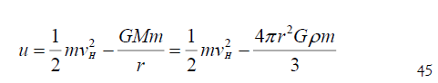
Where r is the radius of the time blast sphere, M is the mass within the time blast sphere and m is the mass of an object. Rearranging and taking k=2u/mc2 as a constant we can derive the red shift dependent Hubble parameter as below:

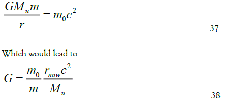
However, from the previous section we believe that the time blast sphere model suggests that G itself is dependent on the radius of the blast sphere and also, we need to take into account relativistic kinetic energy so combining equation 34 and 37 and 26:

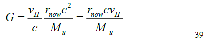
With k being a constant again but this time equal to k=u/mc2. Note that m0 is the mass energy rather than the actual mass in 3D space. It can be thought of as the mass stored in the time dimension as discussed earlier. Also, although we are dealing with a single particle above, if we take m0/m to be the average ratio observed in the universe then vH will represent the global Hubble expansion velocity we observe. If we compare 4.29 with equation 4.10 then k will be zero meaning that the kinetic energy is balanced by the energy stored such that c will always be the escape velocity of the universe.

The above therefore suggests that the expansion rate is entirely due to the amount of matter that has transformed from energy stored in the time dimension into solid matter in 3D space. So, if the process of retardation did not exist, the expansion rate would be a constant (c as it happens). The expansion of the universe observed would be as shown in the diagram for the expansion complete or by Friedman with a constant z relationship i.e., ΩΛ=1. Although we have shown that the presence of matter does not itself drive expansion then the probability of matter colliding or coming together with other matter will be related to the density and type of matter. Therefore, the chances of more matter changing from light to matter will vary according to density. This is simply due to statistics and probability of encountering other particles. The critical thing though is if G is dependent on r then the “starting point” energy form is for expansion of all “matter” to start out at the speed of light, undergo many collisions and then slow down to its current rate.

Dark Matter – Gravity on a Galactic Scale

Observations of the movements and interactions of galaxies has shown that there appears to be too much gravity compared with the light that emanates.[14] When modelled with the amount of gravitational interaction that can be seen from the stars and light observed, then galaxies should simply fall apart. So, something extra is present that is holding them together and the idea of dark matter came about to account for this. In the time blast wave model this might instead come about as an expansion of the above gravity explanation.

Within the blast sphere, then we will observe at any time a thin peeling of the sphere. As objects coalesce and take up more “space” in the time dimension they are then able to interact over a larger part of the blast wave front. The impact of this will be that particles from a more historic part of the blast sphere will now interact with the objects as they grow such that they will grow even further. The more the object grows, the greater its ability would become to borrow matter from an earlier peeling of the blast wave. This would have the effect that the object would effectively grow larger than the matter that initially went into the object from the observable peeling. In other words, localised gravity would become even stronger all by itself as it gathered matter from other previously hidden peelings of the blast sphere. This mechanism is effectively bringing energy and matter into our observation window from an earlier “time” in the blast sphere. So dark matter can perhaps be thought of as the matter shown in the inner grey ring of Figure 2.

When we think about the universal gravity constant then the gravity we feel would already include the mass of all the inner dark matter as it will be within the expansion sphere – so even though we cannot see it, it will still affect the mass we can see.[12]

Note this interaction with matter in an earlier part of the blast sphere might also mean that as objects move and cause a dilation they do not continue to fall away in time from their non- moving counterparts. The wave of matter behind us effectively takes hold of the new matter and propels it forward again to be at or close to the average velocity of time (vH) meaning that the dilation merely causes a distortion in the blast wave front. This effect might not add mass to the visible object in causing this effect - the matter behind us in the blast wave needs room to grow in the dimension of time so may push without ever encroaching into the visible part of the blast wave[13,14].

Dark energy

We have shown above that dark energy is not required to explain an acceleration in expansion of the universe as it does not exist in the time blast sphere model. But there is evidence in the CMB data that suggests that there was a repulsive force present in the early universe that caused CMB photons to have a smaller lensing effect which consequently caused there to be less structure than there might otherwise have been.[15] This could be a result of the push mechanism mentioned at the end of the dark matter section. If this were the case, this would mean that only matter exists behind us and that our presence in time is at the front of the blast wave. Alternatively, this could be evidence for there being hidden matter/energy ahead of us in the blast wave, which would be expected if, as suggested in the Dark Matter section there is matter behind us on the blast wave. It makes sense that in the early universe the matter within the blast sphere was more mixed and able to interact. The CMB data also predicts the presence of dark matter, an attractive force that created structure. The proposed level of structure is 24% dark matter, 4.6% matter and 71.4% dark energy. Returning to Figure 1-if the above ratios are correct this suggests that the thin black band that we are aware of on a day-to-day basis makes up 4.6% of the volume of the blast wave with 24% being behind us (signified by the grey band behind and 74% being in front signified by the outer grey band. So dark energy (and dark matter) may have played a role in terms of creating anisotropy in the otherwise isotropic space. And in the early universe, matter would have been close enough that more mixing would have been possible as the matter swirled around before becoming a predominantly isotropic expansion.

Black holes

In the time blast sphere model, a black hole is just a region of the blast sphere that has dimpled or turned in on itself so severely that light is no longer able to get around it. A black hole will simply behave like an energy well sitting on the surface of the blast sphere with the bottom of the well out of sight but still being pushed forwards in time. As we know whether a mass ends up as a black hole depends on if the matter is compacted into a region smaller than its Schwarzschild radius[16]. If the matter of the object prevents you from getting at the mass’s Schwarzschild radius you will not see it as a black hole – light will bounce off for example or interact with the matter before it can reach that point. Note this well is dependent purely on mass, not density. So, if the object is dense enough that light can reach the point in the well where the sides are steep enough to prevent light getting out then it will appear to us as a black hole. Crucially this model does not suggest that black holes are singularities they are simply areas that are sitting earlier in the blast sphere and are made invisible by the change in the speed of time required to move across the blast wave front.

It is interesting to consider what happens to a black hole as the blast wave continues to expand. As the blast sphere front expands in time, then the matter within the black hole would be stretched. This stretching then will lead to a reduction in the density which will lead it to, at least at the fringes, reach out to a point in the energy well where it can radiate outwards.

The Size and Shape of the Universe

It is perhaps interesting to note that in our spiral model the most distant object as of 2016 in the universe with a redshift of 11.09 would appear to be at around 3094 Mpc, 10.1 billion light years and that this is merely an artefact of the way light rays would emanate from the early universe. In our model the current radius of the blast sphere is only around 95 Mpc leading to a sphere circumference of 5/7 Mpc meaning the universe is smaller than originally thought17. The universe would only appear to be far larger due to the spiralling light path that early photons would take to reach us.

An interesting prospect of this spiral path is that if you look in a certain direction it might be possible to see the same object or at least its historical counterpart more than once. It might even be possible to see a historical version of our own galaxy. It would obviously appear very different because of the time difference and would be difficult to pick out or even know which direction to look in.

Wave Nature of Light and quantum size particles We showed in figure 2 a dark grey band signifying the small “window” of the time spatial dimension we experience. This in a sense signifies the width of our appreciation of the time dimension. It cannot have a zero width though it is likely to be very small. Because it must have a finite size this therefore means that there is a degree of freedom available for any particle we are observing that is smaller than the window itself. For particles that are larger, they will fill the window and any effects would be limited. So let us consider two tiny particles that are smaller than the size of the “window”.

Because of their size, they basically canexist over a range of “times” relative to each other i.e., each particle can either be slightly in front or behind the other in time at the time of interaction. This degree of freedom also opens the possibility that particles can spin or vibrate in the time dimension and consequently store energy in this way. If we return to the blast wave idea and think of photons being caught up in the wave behaving like water molecules in a wave then it is possible that even though in general the blast wave may be moving in a forward direction, the individual particles might be spinning as in Figure 11. So, it is probable that particles caught in the time blast sphere will do the same. The effect would be that a more massive observer might see the small, approaching photon particle phasing in and out of existence as it moves forwards and back in time relative to the observer. i.e., it will display wave like behaviour. But the photon is in fact a particle that is simply spinning in time and will therefore interact with matter as a particle if it collides with it as it does in the photoelectric effect18. If we assume for a moment that the “window” has a prime viewing area at its centre. And around the edges it cannot be fully seen. Then a particle that spins in time will phase in and out of existence i.e., will behave like a wave. The effect is illustrated in Figure 12.

Figure 11: Illustration of orbital path of water molecules within a wave

Figure 12: Visual representation of the effect of a photon spinning in time as it approaches asn observer and the relative intensity observed at key points in the rotation

Time as we perceive it is shown vertically and individual pinpoints of time are shown by the duplicated approaching photons and “eyes”. Distance from the observation point is displayed horizontally. The dashed lines beside each “eye” is the area over which the particle’s existence is appreciated – as stated above an observer’s window of instantaneous observation cannot be of zero size as nothing would be observed, but equally cannot be infinite. This window would have width in both space and time directions and is unlikely to have a “Boolean” effect when dealing with particles of a smaller size compared to the window. What we mean by this is that if an object registers dead centre of the window it would have a larger intensity (be more present as a particle) and if it is off centre it would have a lesser intensity. The time window of appreciation is signified by the dashed parallel lines beside the eye. Note, the observation point signified by the eye is not a solid plate but must be a grating or double slit to appreciate the effect without disturbing it. The photon is a tiny particle, smaller than the window and is shown to be spinning in the time reference frame (vertical). So, when the photon’s spin has it dead centre of the time and space window it has its largest intensity of presence registered. The modelled intensity is shown beside the figure. The phasing in and out of time of a single photon “particle” caused by its spin in the time reference frame can therefore explain how a single photon can interfere in a wave like way with itself. A photon arrives at the double slit but because it phases in and out of time it would dip forward and back in time slightly from our perspective because of its spin. It can therefore arrive/pass through one or the other slits multiple times (as a wave packet) because the double slit would be sitting at an overall fixed effective time (being a large object and not affected at the microscopic level by the individual particles spinning). Consequently, it would be able to interfere with itself as is observed. The above effect would also not be confined to photons but also any small particle such as electrons which are of similar size relative to the “window”. So, by looping around in the time dimension tiny particles can therefore possess both wave and particle like properties. If we now consider for a moment that the “window” is not simply an observational window but creates a confinement space in which the photon or other particle can spin - perhaps because this window is being pushed along by the blast wave of time it forces the particle to spin within the confines of the box. If this is the case, then a quantum effect would be created with only whole multiples of spin being stable within the box.

Conclusions and wider implications

We have presented a model which can explain the observed expansion of the universe whereby time is the metric of expansion which has many effects. Just after the big bang then all energy in the universe existed as radiation which was expelled at the speed of light. The light was so densely packed that the photons collided, adjusted trajectory and then consequently gained mass. The acceleration observed in the initial universe would have caused a battle between individual photons and matter with energy being converted backwards and forwards from mass to radiation, such that a chain effect created the overall average acceleration rate of the universe which rose to an instant peak in velocity of the speed of light and then subsided much like a blast wave would in 3D space. Our model predicts that the universe is decelerating in its expansion contrary to previous conclusions.

Notably this model also sets out a maximum speed for the universe – the speed of light and that photons once they lose a dimension of space must travel at the speed of light. The theory of special relativity came about due to this limit of speed effect being imposed on the universe and everything flowed from this without explaining exactly why the limit had an exact finite value. The mathematics of special relativity specify that the mass of an object will head to infinity when a mass approaches the speed of light, but it does not explain what is so special about the value itself. This theory in contrast effectively explains special relativity from the principal of time expansion which as a result then leads to there being a limit on speed in our universe. The effect of gravity is also described by this theory with the effect that the universal gravitational constant will vary with the size of the universe. Wave-particle duality comes about due to the finite size of the window of time over which we can perceive time.

This hypothesis also raises the question of whether the universe would exist at all if time did not behave in this way. Clearly if we were not moving in the time reference frame, time would not progress forwards so by definition, time would simply not exist. So, expansion is perhaps an inevitable artefact of time procession.

Appendix 1: Exponential Fit for varying expansion rate

As described in the text above to obtain the best correlation with the observed luminosity data we applied a simple exponential decay of the expansion velocity as a function of r, the time blast radius.

The data suggested that there has been a steady decrease in the speed of expansion from z=1.4 through to z=0. To model this decrease we used the following equation:

Where vt+C is the initial velocity of time expansion, r is the blast sphere radius and C is the final velocity the system will reach and equilibrate to. Using the above we were able to accurately model the decrease in velocity for the range of data available to us as seen in Figure 4. Note this does not prove or disprove that this equation accurately describes the decay of the system entirely as we do not have data relating to the very early universe (r<45 Mpc). We used a simple exponential decay to model the system as it is what might be expected if velocity is being reduced by interactions of the particles of the system itself and maybe what you might expect from an expanding system. We do theorize in section 4 that the initial velocity is most likely the speed of light c. If we constrain our fit such that vt+ C=c then reasonable fit can still be obtained although it is not as good at higher z compared to there being no restriction as seen in Figure 13. This might indicate a failing in the simple exponential decay function to accurately predict the decay that occurred over all timeFigure 14.

Figure 13: Duplication of Figure 4 with addition of model results for decay from vH=c.

Figure 14: Exponential decay curves as described in the text

It might be that the decay mechanism was initially much sharper going from the speed of light to around 5 or 6% of the speed of light almost instantly and then gradually continued to decrease from there. Other models and studies have suggested that there was an initial rapid expansion period, called inflation20,21.

Results of fit allowing freedom in vt+C resulted in vt/c = 0.0358, r = 95.053Mpc, k=0.0313, C=0.0200

Results of fit restricting vt+C=v resulted in vt/c = 0.9771, r=95.053Mpc, k=0.1103, C=0.0229 (deliberately keeping r the same as above fit).

References

1. Hubble EP. The observational approach to cosmology. Oxford: Clarendon Press; 1937.
   Google Scholar                   Crossref
2. Einsten A, Infeld L. The Evolution of Physics: From Early Concepts to Relativity and Quanta. USA: S imin & S chuster.1938;1(9):7.
   Google scholar                      Crossref
3. Planck Collaboration. 2016 Planck 2015 results XIII. Cosmological parameters. A&A 594, A13; 2016 (doi:10.1051/0004-6361/201525830)
4. Riess AG, Casertano S, Yuan W. Large Magellanic Cloud Cepheid standards provide a 1% foundation for the determination of the Hubble constant and stronger evidence for physics beyond ΛCDM. Astrophys J. 2019;876(1):85.
   Google Scholar                          Crossref 
5. Hotokezaka K, Nakar E, Gottlieb O et al . A Hubble constant measurement from superluminal motion of the jet in GW170817. Nat  Astron. 2019 ;3(10):940-44.
   Googlescholar                              Crossref
6. Aghanim N, Akrami Y, Ashdown M et al. Planck 2018 results-VI. Cosmological parameters. Astron Astrophys. 2020 ; 641.
   Google Scholar              Crossref
   
7. Collaboration P, Aghanim N, Akrami Y et al . Planck 2018 results VI. Cosmological parameters.
   Google scholar                            Crossref
8. Mukherjee S, Ghosh A, Graham MJ et al. First measurement of the Hubble parameter from bright binary black hole GW190521.arXiv:2009.14199.
   Google scholar                               Crossref
9. Riess AG. Observational evidence from supernovae for an accelerating universe and a cosmological constant Astronomical.J.1998;1009.
   Google scholar                              
10. SDSS collaboration, Betoule M. Improved cosmological constraints from a joint analysis of the SDSS-II and SNLS supernova samples Astron. Astrophys. 568. A22 [1401.4064] Crossref Preprint; 2014.
    Google scholar                                 Crossref
11. Oesch PA, Brammer G, Van Dokkum PG et al. A remarkably luminous galaxy at z= 11.1 measured with Hubble Space Telescope grism spectroscopy. Astrophys J. 201;819(2):129.
    Google scholar                    Croossref
12. Pike OJ, Mackenroth F, Hill EG, Rose SJ. A photon–photon collider in a vacuum hohlraum. Nat Photon. 2014;8(6):434-6.
    Google scholar                      Crossref
13. Cowen R. Andromeda on collision course with the Milky Way. Astrophys J .2012;31;1:3.
    Google scholar                     
14. Trimble V. Existence and nature of dark matter in the universe. Annual review of astronomy and astrophysics. 1987;25(1):425-72.
    Google scholar         Crossref
15. Spergel DN, Verde L, Peiris HV et al . First-year Wilkinson Microwave Anisotropy Probe (WMAP)* observations: determination of cosmological parameters. Astrophys J Suppl Ser. 2003;148(1):175.
    Google scholar              
16. Schwarzschild K. Uber das Gravitationsfeld eines Massenpunktes nach der Einstein'schen Theorie. Berlin. Sitzungsberichte.1916;18.
    Google scholar                 Crossref